If you’re working with an Excel pivot table, you might want to select a specific section, such as the subtotals, so you can apply formatting. The short video below has a few pivot table selection tips.
Video: Select Specific Parts of Pivot Table
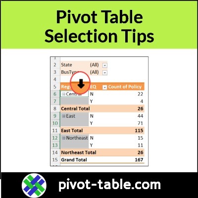
Do you want to select one or two subtotal lines in a pivot table, and change those to a different font or fill colour? Perhaps you want to make one sales region’s totals stand out from the others, in a monthly pivot report.
In this short video, I show how to select specific sections of an Excel Pivot Table, by using the Selection Arrow feature.
And, if the Selection Arrow doesn’t appear on your computer, you’ll see how to turn that feature on, with just a couple of clicks.
Video Timeline
0:00 Introduction
0:15 Pivot Table Selection Arrow
0:47 Select Subtotal Rows
1:06 Select Labels and Values
1:59 Change Enable Selection Setting
More Pivot Table Formatting Tips
Here are a few links to my Contextures site, where you can get more pivot table formatting tips and videos.
Number Formatting: There’s a special way to format numbers in a pivot table, if you want that formatting to stick. If you format pivot table number the same way as normal worksheet cells, the number formatting might disappear, when you refresh the pivot table.
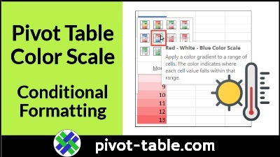
Conditional Formatting: Pivot Table conditional formatting needs an extra step, after you set it up. If you miss that step, new data might not show the conditional formatting!
Pivot Table Styles: An efficient way to format pivot tables is to make changes to the built-in pivot table styles, or create your own custom pivot table styles.
Excel pivot tables don’t show hyperlinks, but there’s a way around that problem! In the video below, you’ll see how to create fake clickable hyperlinks in a pivot table, by using a few lines of Excel VBA code, and a bit of formatting.
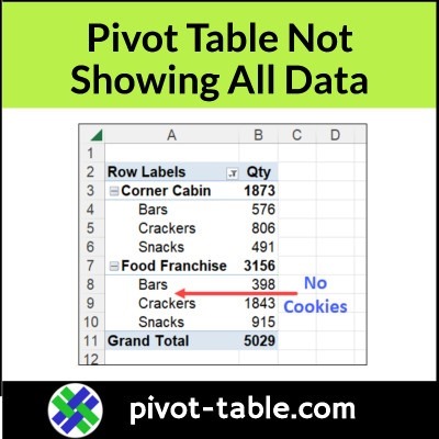
Pivot tables are great for summarizing data, but do you ever notice that there are missing items in a pivot table?
For example, you know there are product records in the source data table, but one product isn’t showing up in the pivot table. How can you troubleshoot and fix the problem to show all data?
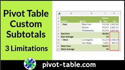
In an Excel pivot table, subtotals are automatically added to the outer fields, when you add more fields below them. You can also add extra subtotals, if needed, by creating custom subtotals for a pivot field. There are some limitations though, which you can see in the video and notes below. Continue reading “Excel Pivot Table Custom Subtotal Limitations”
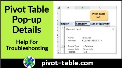
If Excel error messages appear when you try to refresh a pivot table, there are macros on my Contextures site that can help you troubleshoot those problems. I’ve just added another macro on that page, to show a pop-up message with details, if a specific pivot table is behaving badly.
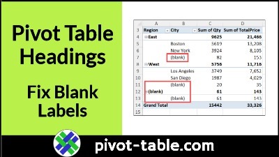
After you build an Excel pivot table, you might see a few row labels or column labels that contain the text “(blank)”.
This happens when data is missing from the source data. For example, in the source data, you might have a few sales orders that don’t have a Store number entered.
Video: Fix Pivot Table Headings
Watch this short video to see how to fix those “(blank)” labels, and there are written steps below the video.
In the pivot table shown below, there are three City heading cells, in column B, that shows (blank), instead of a city name. There is also one Region heading cell in column A that has the same problem.
When working with a pivot table, I find that text distracting, and usually remove it, to get a cleaner look in the pivot table.
Sometimes I replace the “(blank)” with other text, such as “N/A”
In most cases, I want the cell to look blank, so I replace it with a space character
The steps to do that are below this screen shot.
Pivot Option Setting Does NOT Change Labels
First, here’s a solution that you might have tried, to remove the “(blank)” text, and found that it didn’t do what you needed.
In the PivotTable Options dialog box, on the Layout & Format tab, there is a setting, “for empty cells show:”
Maybe you typed “N/A” in that box, or a space character, hoping it would solve the “(blank)” label problem
After making that change in the Options window, you clicked the OK button.
Why That Does NOT Work
After the PivotTable Options dialog box closed, you’d be disappointed to see that the “(blank)” headings were still in the row labels.
That solution does not work for “(blank)” cells, because: that “empty cells” setting has these limitations:
it only affects cells in the Values area
it does NOT affect the Row or Column Labels areas.
For example, in the screen shot below, you can see that:
missing data in the Values area has been replace by N/A
row labels and column labels haven’t changed – they still show “(blank)”.
Manually Change Blank Labels
Instead of using the PivotTable Options, you can manually change the (blank) labels in the Row or Column Labels areas by typing over them in the pivot table.
However, this technique has a couple of limitations too:
You cannot type an existing item name, to replace the (Blank) entry
If you type an existing name, the (blank) label will move into the place where that item was in the pivot table layout
You cannot clear the cell and leave it empty – it must have a text entry
How to Change Label Text
Here are the steps for manually changing a pivot table row label text, or heading labels in the column areas.
Note: I used “N/A” in this example, but you could use a different text string, or a space character.
To change a blank label cell to “N/A”, follow these editing steps:
First, select one of the Row or Column Labels that contains the text (blank)
Even if there are multiple cells with a “(blank)” label, you only need to select one of them.
You DO NOT need to press Ctrl and select all of them
Next, on your keyboard, type N/A in the cell, and then press the Enter key.
Pivot Table Changes
After you press the Enter key, you’ll see the following changes in the pivot table, shown in the screen shot below:
All other (Blank) items in that same pivot field will change to display the same text
In this example, all “(blank)” cells in the City column have changed to “N/A”.
Blank items in other pivot fields are NOT affected
In this example, the “(blank)” cell in the Region column has NOT changed to “N/A”.
It’s November, a month when we expect cooler temperatures here in Canada. However, it was more like summer last weekend, and we enjoyed an afternoon beverage on the patio. Was that normal? What were the November temperatures over the past few years? Let’s use a pivot table with conditional formatting, to find out!
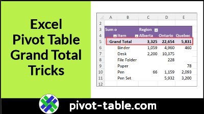
Excel automatically adds grand totals to a pivot table, if there are multiple items in the row area, or in the column area. See how you can change the automatic grand total headings (sometimes), and quickly remove grand totals if you don’t need them.
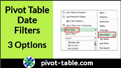
After you create a pivot table in Excel, you can filter the data, to focus on specific things. Maybe you want a top product report, or a regional summary, or see the sales to a couple of new customers. You can also use filters on date fields, and there are 3 different types you can use.
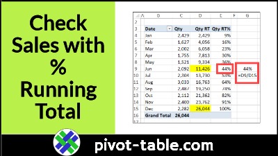
Quickly check your sales results over time, or by top products, with the % Running Total feature in an Excel pivot table. This feature is available in Excel 2010, and later versions.


 in pivot table")