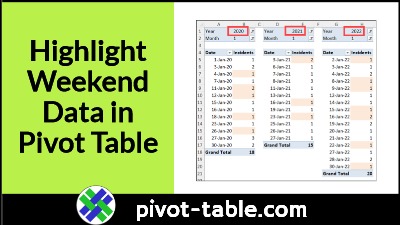
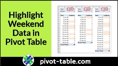
Pivot Table Highlight Weekend Data Conditional Formatting

You can use conditional formatting in an Excel pivot table, to highlight specific data, such as months with high sales numbers. This example uses conditional formatting to highlight the pivot table values that are connected to weekend dates.

Pivot Table Dates and Numbers

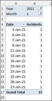
This pivot table has workplace safety data, from a fictitious company.

You can get the sample Excel file on my Contextures site

I’d like conditional formatting to highlight the weekend data:

number of incidents in column B
if the date in column A falls on a weekend.

Get the Weekday Number

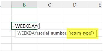
To find out which dates occur on a weekend, you can use the Excel WEEKDAY function.

The WEEKDAY function returns a number, based on a date.
You can also use its optional second argument, return_type, to tell Excel how to number the weekdays.

Test on the Worksheet

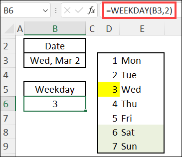
I like to test conditional formatting formulas on a worksheet first, so there’s a date in cell B3, in the screen shot below.

Here’s the formula in cell B6.

=WEEKDAY(B3,2)

That formula checks the date in cell B3.

The return_type argument (2), tells Excel to number the weekdays:

from Monday (1)
to Sunday (7)

Check for Weekend Dates

Next, to check for weekend dates, I can add a test for weekday numbers “greater than 5”

=WEEKDAY(B3,2)>5

That’s the formula I’ll use to set up the pivot table conditional formatting

Apply Conditional Formatting to Pivot Table

Next, follow these steps to apply the weekend highlighting in the pivot table:

Select all the Incidents cells where conditional formatting should be applied

Cells B5 to B20 in this example.

On the Ribbon, click the Home tab, then click Conditional Formatting.
Click New Rule, to open the New Formatting Rule dialog box
In the Select a Rule Type list, click Use a formula to determine which cells to format.
In the Formula box, enter a formula to check the weekday for the date in the first data row:
- =WEEKDAY($B5,2)>5
Click the Format button, and select a Fill colour, then click OK.
Click OK to close the New Formatting Rule dialog box.

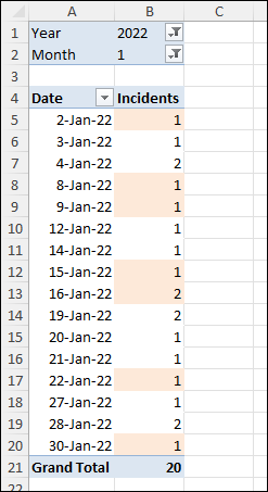
I chose light orange fill colour, and all the weekend incident numbers are highlighted

There’s one more important step though, so be sure to read the next section!

Extra Step for Pivot Table Conditional Formatting

The conditional formatting looks good now, but if you change the pivot table layout, or add new data, the correct cells might not be formatted.

Follow these steps to adjust the conditional formatting rule, so it refers to the pivot fields, instead of a specific range of cells

Select a cell in the pivot table cell
Next, on the Ribbon’s Home tab, click Conditional Formatting, then Manage Rules
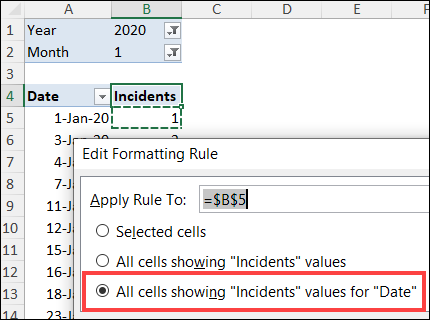
Click on the Weekend rule, and click Edit Rule, to open the Edit Formatting Rule window.
In the Apply Rule To section, click on the 3rd option
All cells showing “Incidents” values for “Date”
Click OK, to apply the revised rule

Highlight Pivot Table Cells With Conditional Formatting

This video shows the steps for applying conditional formatting to pivot tables cells.

Then adjust the rule, so new cells are formatted if the pivot table layout changes.

You can go to my Contextures website for more information on Pivot Table Conditional Formatting, and to get the Excel workbook.

Highlight Weekend Dates in Excel

This video shows the steps for setting up conditional formatting to highlight weekend dates, by using the Excel WEEKDAY function.

NOTE: This example applies conditional formatting on normal worksheet cells. Remember to do the extra step, if you’re using this technique on Excel pivot table cells.

Go to my Contextures site for more information on the Excel Date function, such as WEEKDAY.