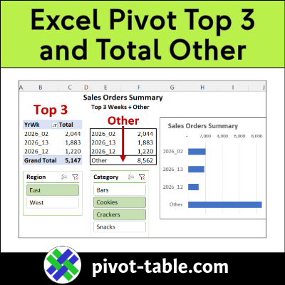
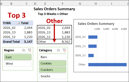
In a short video below, I show how to set up an Excel pivot table with the top 3 items, and a total for all the remaining items, grouped as “Other”.
Continue reading “Excel Pivot Table Filter – Show Top 3 and Total Other”
by contextures.com

In a short video below, I show how to set up an Excel pivot table with the top 3 items, and a total for all the remaining items, grouped as “Other”.
Continue reading “Excel Pivot Table Filter – Show Top 3 and Total Other”
Pivot tables let you summarize thousands of rows of data, with just a few clicks. If you want to focus on a specific part of that summarized data, here are a couple of pivot table filter tricks.
Continue reading “Quick Pivot Table Filter Trick: Hide or Show Items”
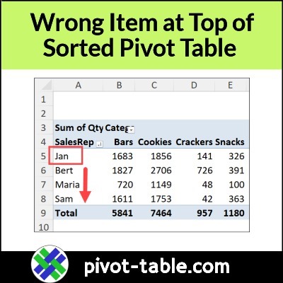
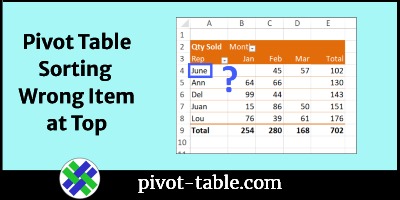
After you sort an Excel pivot table, the wrong item might appear at the top of a column. For example, in the screen shot below, the list of Sales Rep names has Jan at the top. Below that name, all the other names are sorted in the correct alphabetical order.
Continue reading “Wrong Item at Top of Sorted Pivot Table in Excel”
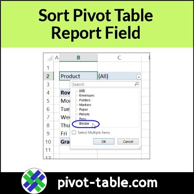
If you have a report filter at the top of your pivot table, do the items in the drop down list ever appear out of order? That happens in my pivot tables occasionally, and there isn’t a quick and easy way to fix the problem!
After you set up a pivot table, you might want to discourage people from filtering the pivot fields, which could hide some of the data. This video shows a couple of ways hide the drop down arrows in the pivot table headings.
Continue reading “Hide Drop-Down Arrows in Excel Pivot Table”
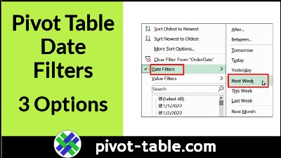
After you create a pivot table in Excel, you can filter the data, to focus on specific things. Maybe you want a top product report, or a regional summary, or see the sales to a couple of new customers. You can also use filters on date fields, and there are 3 different types you can use.
Continue reading “Pivot Table Date Field Filters – 3 Types to Try”
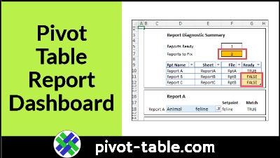
Do you create weekly or monthly reports based on pivot tables, and share those reports with clients or co-workers? If there are multiple pivot tables in your report, use this Excel dashboard technique to check all the filters, before you hit Send!
Continue reading “Excel Dashboard Check Pivot Table Filters Before Printing”
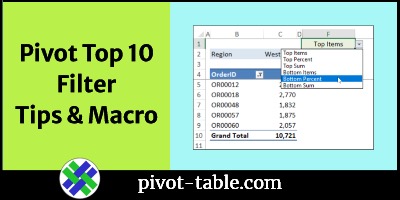
The Pivot Table Top 10 Filter feature lets you focus on what’s working well. Create a report that shows sales from the top regions, or show the best-selling products. You can use this feature to show the opposite too. Which products are selling poorly? Which cities or regions aren’t doing well? These two short videos show quick ways to analyse sales data with pivot table top 10 filters.
Continue reading “How to Use Pivot Table Top 10 Filters to Analyse Sales Data”
Usually, it’s easy to sort an Excel pivot table – just select one of the sort options – A to Z or Z to A – in the heading drop downs. However, you might run into a pivot table sorting problem, where the wrong item stays at the top. See why that happens, and how you can fix the pivot sort problem.
Continue reading “Pivot Table Sorting Problem Wrong Item at Top”
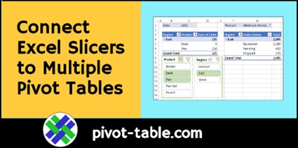
If you create two or more pivot tables from the same source data (pivot cache), you can connect them to the same Excel Slicers. That will make it easy to filter all the connected pivot tables at the same time.
Continue reading “Connect Excel Slicers to Multiple Pivot Tables”