It’s November, a month when we expect cooler temperatures here in Canada. However, it was more like summer last weekend, and we enjoyed an afternoon beverage on the patio. Was that normal? What were the November temperatures over the past few years? Let’s use a pivot table with conditional formatting, to find out!
Get the Temperatures
Every morning, I get check the weather forecast on the Government of Canada Weather page. Will this be a perfect day to stay indoor and work on a pivot table? Usually, the answer is “Yes!”
I also record each day’s min and max temperatures in an Excel table. You can read more about my weather records on my Contextures blog.
You can also get interesting facts about our Canadian weather!

Colour the Temperatures
In that Excel table, there’s a conditional formatting color scale on each column, to give a quick overview of hot and cold days. Because everyone does that, right? ![]()
Here are the highs and lows from last week. And it’s interesting that 13° is blue in the Max column, but dark pink in the Min column.

Compare Temperatures By Year
To compare the November temperatures over the past few years, I created a pivot table from my daily temperature table.
In the pivot table layout, I put:
- Day number in the Rows area
- Year in the Columns area
- Max temperature in the Values area
- Month number in the Filter area
Next, I selected 11 in the filter drop down, to see November temperatures only.
Then, in the Day field, I filtered the Label values, to show only the day numbers from 1 to 14.
Colour the Pivot Table
The next step was to add conditional formatting to all the temperature values, so it’s easy to spot the hot days, and cold days.
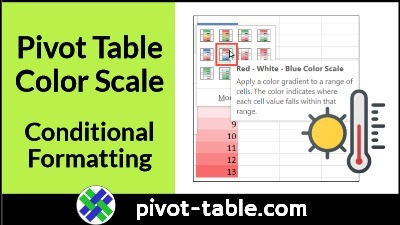
I selected all the temperature values, and applied the Red – White – Blue Color Scale option.
With that option, the high number are red (hot), and low numbers are blue (cold).

And here’s the result, showing early November temperatures for the years 2017 to 2022.
The colours show that this year had the hottest day, and it was much colder back in November 2019!

Adjust Conditional Formatting Rule
In my November weather pivot table, the conditional formatting looks good, and is applied correctly to all the temperature cells.
However, if I change the pivot table layout later, or decide to show a few more days, things might not look so good!
If you apply conditional formatting to a pivot table, there’s an extra step to do, and the video below shows you that step.
You’ll see how to go into the Conditional Formatting Rules, and change the “Apply Rule To” setting, so it refers to the pivot field names, instead of the cell addresses
There are written steps for changing the pivot table conditional formatting rule on my Contextures website.
Video: Pivot Table Data Bars
This video shows another way to use conditional formatting in an Excel pivot table. This example uses data bars, for a quick overview of sales data.
See the setup details and get the sample file for this example.
Video: Temperature Color Scale
This video shows another example of using a conditional formatting color scale to highlight low and high temperatures. This is set up in a named Excel table, instead of a pivot table.
See the setup details for this example, on my Contextures Excel blog.
________________
Conditional Formatting Excel Pivot Table Color Scale

________________