After you create an Excel pivot table, the source data usually changes. New records are added, and old records might be changed or deleted.
Later, when you refresh the pivot table, you should see a summary of your updated data, but sometimes there’s a problem – old data sticks in the drop down lists.
Example: Region Names Changed
To show this pivot table problem, I made short video, which you can see in the next section.
My sample file has data from a fictional sales company, and the source data was changed:
- Central region was merged into the East region.
- Sales records were changed from Central to East
After making those changes, I refreshed the pivot table. As expected, the Central region’s name disappeared from the Region headings.
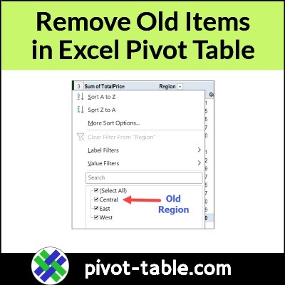
However, Central still shows up in the Region drop down.

Video: Clear Old Pivot Table Items
In this short video, I show how you can clear the old Region name from the pivot table drop down list.
Doing this will also prevent old items from appearing in this pivot table, in the future.
Video: Clear Old Items – Default Settings
In Excel 365, and Excel 2019, it’s even easier to avoid old items in pivot table drop downs.
Instead of changing this setting for every pivot table that you create, you can change it once, in your Excel default settings for Pivot Tables.
In the video below, I show the steps for changing an individual pivot table, like I did in the previous video.
Then, at the 2:57 mark, I show how to change the default setting, in Excel 365. You can skip to that section, if you’d like!
Prevent Old Items in Pivot Table
To stop old items from showing in an existing pivot table, follow the steps below.
NOTE: This setting will affect all the pivot tables that use the same pivot cache.
- First, right-click a cell in the pivot table
- Next, in the right-click pop-up menu, click on PivotTable options
- In the PivotTable Options dialog box, click on the Data tab
- In the Retain Items section, there is a drop down for “Number of items to retain per field”
- By default, that is set to Automatic.
- Click the drop down arrow, and select None from the drop down list.
- Click OK, then refresh the pivot table.

Get the Excel Workbook
To get the sample file, go to the Clear Old Items page on my Contextures site.
That page also has Excel macros that you can use, to
- change the Retain Item settings for all pivot tables in the workbook
- change Excel’s default settings for pivot tables (Office 365 or Excel 2019 and later)
More Pivot Table Tutorials
_______________________
Remove Old Items – Excel Pivot Table Drop Down

_______________________