If you add times to an Excel Pivot Table, and format the time to show tenths of a second or hundredths of a second, zeros might appear after the decimal point.
The decimals for tenths of a second or hundredths of a second are rounded to zero, and changing the pivot table number format does not fix the problem.
Pivot Table Zero Decimals
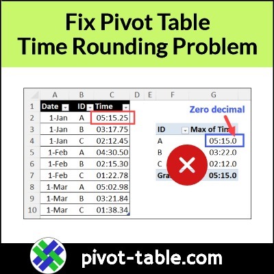
In the screen shot below, I’ve highlighted the problem in the pivot table time column.
- maximum time for the A team is 5:15:25 – 5 minutes, and 15 and 25 hundredths seconds
- pivot table shows the time as 5:15:0 – 5 minutes, and 15 seconds
Instead of rounding the decimal to 2, it rounded to zero.

Video: Fix Pivot Table Time Rounding Problem
In the video below, I show how this time rounding problem can happen, and the steps to fix the problem.
There are written steps below the video, and more details on my Contextures site, on the Pivot Table Time Fields page.
Video Timeline
- 0:00 Introduction
- 0:12 Build a Pivot Table
- 0:55 Format the Time
- 1:38 Fix the Time Problem
- 2:43 Format the New Field
Fix Pivot Table Time Rounding Problem
To fix the pivot table times, so they show tenths of seconds and hundredths of seconds, you can use a simple workaround.
To begin, follow these steps to add a column in the source data:
- First, add a new column in the pivot table source data–in this example, TimeCalc
- Next, in the new column, enter a formula with a simple link to the original time value cell in that row.
- In the screen shot below, cell D2 has this formula: =C2
- If the source data is in a named Excel table, the formula should automatically fill down to the last row.
- Leave the new column in General format – do NOT change it to a time format

Add New Field to Pivot Table
After you add the new column to the source data, follow the steps below, to update the pivot table.
- To refresh the pivot table, right-click on a pivot cell, and click the Refresh command
- The new field will appear in the pivot table field list, where you can drag it to the pivot table’s Values area.
- To show the maximum times, right-click on one of the new values, click Summarize Values by, and then click Max
Format as Time With 2 Decimals
Next, follow the steps below to format the times:
- First, right-click on any cell in new pivot value column, and click the Value Field Settings command
- Click the Number Format button, and click on the Custom category at the left.
- To show the times with 2 decimal places, format the values with this custom number format: m:ss.00
- This time format shows tenths of a second, or hundredths of a second.
- Click the OK button to apply the formatting
The numbers are formatted correctly in the new field, tenths of a second, and hundredths of a second
To complete the changes, you can remove the original time field, which had the rounded tenths of a second or hundredths of a second, showing a zero instead of the correct numbers.

Get the Excel Workbook
To get the sample Excel file that I used in the video, go to my Contextures site, on the Pivot Table Time Fields page. The zipped file is in xlsx format, and does not contain any macros.
____________________
Fix Excel Pivot Table Time Rounding Problem

____________________