If you add times to an Excel Pivot Table, and format the time to show tenths of a second or hundredths of a second, zeros might appear after the decimal point.
The decimals for tenths of a second or hundredths of a second are rounded to zero, and changing the pivot table number format does not fix the problem.
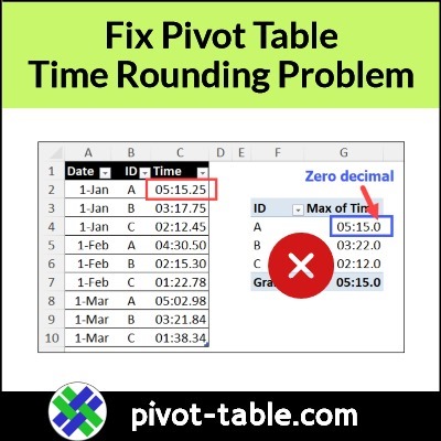
Pivot Table Zero Decimals
In the screen shot below, I’ve highlighted the problem in the pivot table time column.
maximum time for the A team is 5:15:25 – 5 minutes, and 15 and 25 hundredths seconds
To fix the pivot table times, so they show tenths of seconds and hundredths of seconds, you can use a simple workaround.
To begin, follow these steps to add a column in the source data:
First, add a new column in the pivot table source data–in this example, TimeCalc
Next, in the new column, enter a formula with a simple link to the original time value cell in that row.
In the screen shot below, cell D2 has this formula: =C2
If the source data is in a named Excel table, the formula should automatically fill down to the last row.
Leave the new column in General format – do NOT change it to a time format
Add New Field to Pivot Table
After you add the new column to the source data, follow the steps below, to update the pivot table.
To refresh the pivot table, right-click on a pivot cell, and click the Refresh command
The new field will appear in the pivot table field list, where you can drag it to the pivot table’s Values area.
To show the maximum times, right-click on one of the new values, click Summarize Values by, and then click Max
Format as Time With 2 Decimals
Next, follow the steps below to format the times:
First, right-click on any cell in new pivot value column, and click the Value Field Settings command
Click the Number Format button, and click on the Custom category at the left.
To show the times with 2 decimal places, format the values with this custom number format: m:ss.00
This time format shows tenths of a second, or hundredths of a second.
Click the OK button to apply the formatting
The numbers are formatted correctly in the new field, tenths of a second, and hundredths of a second
To complete the changes, you can remove the original time field, which had the rounded tenths of a second or hundredths of a second, showing a zero instead of the correct numbers.
Get the Excel Workbook
To get the sample Excel file that I used in the video, go to my Contextures site, on the Pivot Table Time Fields page. The zipped file is in xlsx format, and does not contain any macros.
In a perfect world, if you need to make a pivot table, the data is nicely organized in a table, and you can connect to that, quickly and easily.
Unfortunately, as you know, things aren’t always perfect, especially when it comes to data! And sometimes the data is in two or more separate tables, so you need to combine it somehow, before you can build a pivot table..
4 Ways to Combine Data for Pivot Table
There are different ways you can combine data from multiple tables in Excel. For example:
Power Query
VSTACK Formula
Excel Macros
Pivot Table Wizard
Combine Data Videos
In the sections below, there are a couple of short “Combine Data” videos that I’ve made recently.
The first video shows how to use the VSTACK function, which is available in Excel 365. It returns multiple ranges in a vertical stack, so it’s easy to combine tables that have identical structures.
The second video shows how to combine data using the old Pivot Table Wizard. It creates a pivot table with several limitations, but it might do what you need – if you don’t need anything fancy!
create named range for VSTACK formula cell spill range
Video: Create Pivot Table from 2 Tables
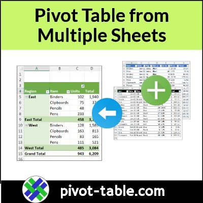
Here’s the VSTACK function video, in which I combine the data from tables on 2 separate worksheets. It only takes one cell with a formula, to return all the data from the two tables.
I included the headings for the first table too, because pivot table data needs headings!
Video Timeline
00:00 Pivot Table from Multiple Sheets
00:20 VSTACK Function
00:52 VSTACK Formula
01:21 Combined Data
01:39 Named Range
02:11 Add Pivot Table
Pivot Table Wizard
What if you don’t have Power Query, or the Excel VSTACK function. And you don’t want to use Excel macros?
In that case, you can use the old Pivot Table Wizard to do the job. It’s well hidden in newer versions of Excel, but in the video, I’ll show you how to open it, with an Excel keyboard shortcut.
Video Timeline
0:00 Data on 2 Sheets
0:24 Open PivotTable Wizard
0:50 Select Sheet Ranges
1:08 Page Field Settings
1:29 Adjust the Pivot Table
2:04 Show Sum
2:15 Page Field
Get the Sample File
For all 4 methods to combine data, you can find detailed steps, and sample files, on my Contextures site.
When you create a pivot table, and select a cell in it, a pivot table field list usually appears, at the right side of the Excel window. See how you can adjust that list’s layout, width, and position. Also, see how we moved pivot fields in the olden days – do you remember the PivotTable Wizard?
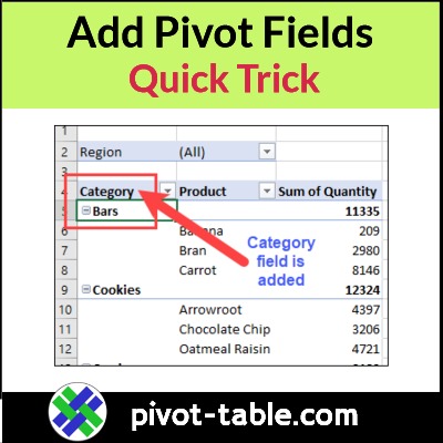
After you press Enter, the pivot table layout changes.
The field that you typed moves into the active cell.
The existing fields shift down, and the added field takes its new position.
pivot field added to worksheet layout
More Tips for Moving Labels
The first video above shows how to move pivot fields.
You can use a similar trick to move the pivot items in a pivot table.
The short video below shows how to move the Excel pivot items, and you can find written steps on the Move Pivot Table Labels page on my Contextures site.
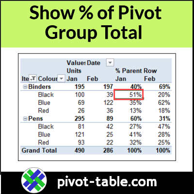
In an Excel pivot table, you can use Excel’s built-in custom calculations, for a different view of the data.
For example, in the video below, I set up a pivot table to show what % of a company’s monthly sales were Binders. Also, what % of Binder sales was for each colour – red, blue, and black.
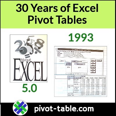
On Saturday, it’s the 38th anniversary of Microsoft Excel, which was released on September 30th, 1985. Eight years later, sometime in 1993, Pivot Tables were added, in Excel 5.0! Happy 30th Anniversary to Excel Pivot Tables.
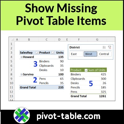
By default, the Pivot Table shows only the items for which there is data. In the example shown in this video, not all colours were sold to each customer. You may wish to see all the items for each customer, even those items with no data.
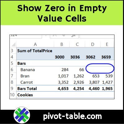
If you build an Excel pivot table, and no data is entered for some items, there will be blank cells in the pivot table values area. See how to change those blanks to zero, or a text string, such as “N/A”
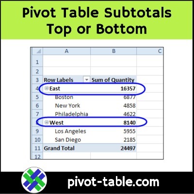
When you create a new pivot table, and add multiple fields to the row or column area, subtotals are automatically created. For Row fields the automatic subtotals usually appear at the top, and you can move them to the bottom, if that’s your preference. There are a few limitations though, which you can see in the video and the written notes below.