
If you have a report filter at the top of your pivot table, do the items in the drop down list ever appear out of order? That happens in my pivot tables occasionally, and there isn’t a quick and easy way to fix the problem!
Author: Debra
Remove Old Items – Excel Pivot Table Drop Down
After you create an Excel pivot table, the source data usually changes. New records are added, and old records might be changed or deleted.
Later, when you refresh the pivot table, you should see a summary of your updated data, but sometimes there’s a problem – old data sticks in the drop down lists.
Example: Region Names Changed
To show this pivot table problem, I made short video, which you can see in the next section.
My sample file has data from a fictional sales company, and the source data was changed:
- Central region was merged into the East region.
- Sales records were changed from Central to East
After making those changes, I refreshed the pivot table. As expected, the Central region’s name disappeared from the Region headings.
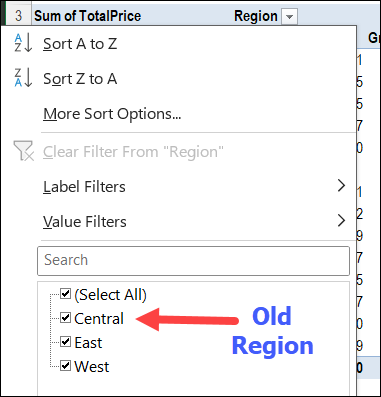
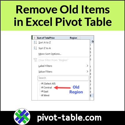
However, Central still shows up in the Region drop down.
Video: Clear Old Pivot Table Items
In this short video, I show how you can clear the old Region name from the pivot table drop down list.
Doing this will also prevent old items from appearing in this pivot table, in the future.
Video: Clear Old Items – Default Settings
In Excel 365, and Excel 2019, it’s even easier to avoid old items in pivot table drop downs.
Instead of changing this setting for every pivot table that you create, you can change it once, in your Excel default settings for Pivot Tables.
In the video below, I show the steps for changing an individual pivot table, like I did in the previous video.
Then, at the 2:57 mark, I show how to change the default setting, in Excel 365. You can skip to that section, if you’d like!
Prevent Old Items in Pivot Table
To stop old items from showing in an existing pivot table, follow the steps below.
NOTE: This setting will affect all the pivot tables that use the same pivot cache.
- First, right-click a cell in the pivot table
- Next, in the right-click pop-up menu, click on PivotTable options
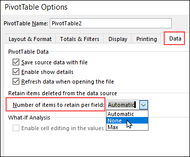
- In the PivotTable Options dialog box, click on the Data tab
- In the Retain Items section, there is a drop down for “Number of items to retain per field”
- By default, that is set to Automatic.
- Click the drop down arrow, and select None from the drop down list.
- Click OK, then refresh the pivot table.
Get the Excel Workbook
To get the sample file, go to the Clear Old Items page on my Contextures site.
That page also has Excel macros that you can use, to
- change the Retain Item settings for all pivot tables in the workbook
- change Excel’s default settings for pivot tables (Office 365 or Excel 2019 and later)
More Pivot Table Tutorials
_______________________
Remove Old Items – Excel Pivot Table Drop Down
_______________________
Quick Count Unique (Distinct) Items in Excel Pivot Table
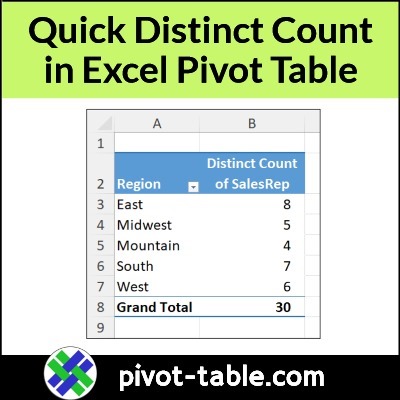
It’s easy to get a sum in a pivot table, or a total count. But how can you count unique items in an Excel pivot table?
For example, if you’re analyzing sales data, you might need to show these types of counts:
–How many unique products were sold in each store?
–How many distinct people made sales in each region?
Continue reading “Quick Count Unique (Distinct) Items in Excel Pivot Table”
Fix Excel Pivot Table Time Rounding Problem
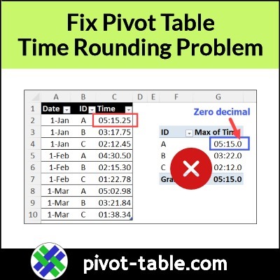
If you add times to an Excel Pivot Table, and format the time to show tenths of a second or hundredths of a second, zeros might appear after the decimal point.
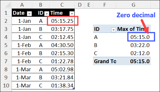
The decimals for tenths of a second or hundredths of a second are rounded to zero, and changing the pivot table number format does not fix the problem.
Pivot Table Zero Decimals
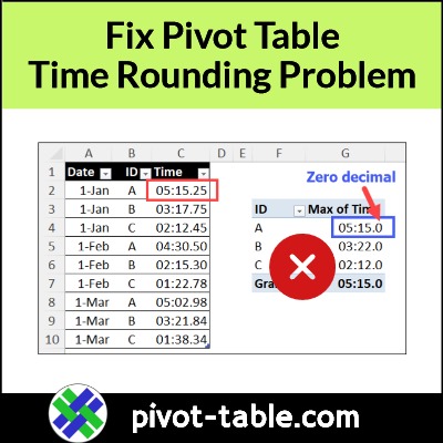
In the screen shot below, I’ve highlighted the problem in the pivot table time column.
- maximum time for the A team is 5:15:25 – 5 minutes, and 15 and 25 hundredths seconds
- pivot table shows the time as 5:15:0 – 5 minutes, and 15 seconds
Instead of rounding the decimal to 2, it rounded to zero.
Video: Fix Pivot Table Time Rounding Problem
In the video below, I show how this time rounding problem can happen, and the steps to fix the problem.
There are written steps below the video, and more details on my Contextures site, on the Pivot Table Time Fields page.
Video Timeline
- 0:00 Introduction
- 0:12 Build a Pivot Table
- 0:55 Format the Time
- 1:38 Fix the Time Problem
- 2:43 Format the New Field
Fix Pivot Table Time Rounding Problem
To fix the pivot table times, so they show tenths of seconds and hundredths of seconds, you can use a simple workaround.
To begin, follow these steps to add a column in the source data:
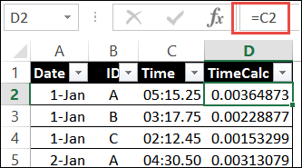
- First, add a new column in the pivot table source data–in this example, TimeCalc
- Next, in the new column, enter a formula with a simple link to the original time value cell in that row.
- In the screen shot below, cell D2 has this formula: =C2
- If the source data is in a named Excel table, the formula should automatically fill down to the last row.
- Leave the new column in General format – do NOT change it to a time format
Add New Field to Pivot Table
After you add the new column to the source data, follow the steps below, to update the pivot table.
- To refresh the pivot table, right-click on a pivot cell, and click the Refresh command
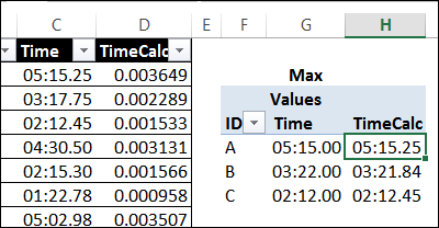
- The new field will appear in the pivot table field list, where you can drag it to the pivot table’s Values area.
- To show the maximum times, right-click on one of the new values, click Summarize Values by, and then click Max
Format as Time With 2 Decimals
Next, follow the steps below to format the times:
- First, right-click on any cell in new pivot value column, and click the Value Field Settings command
- Click the Number Format button, and click on the Custom category at the left.
- To show the times with 2 decimal places, format the values with this custom number format: m:ss.00
- This time format shows tenths of a second, or hundredths of a second.
- Click the OK button to apply the formatting
The numbers are formatted correctly in the new field, tenths of a second, and hundredths of a second
To complete the changes, you can remove the original time field, which had the rounded tenths of a second or hundredths of a second, showing a zero instead of the correct numbers.
Get the Excel Workbook
To get the sample Excel file that I used in the video, go to my Contextures site, on the Pivot Table Time Fields page. The zipped file is in xlsx format, and does not contain any macros.
____________________
Fix Excel Pivot Table Time Rounding Problem
____________________
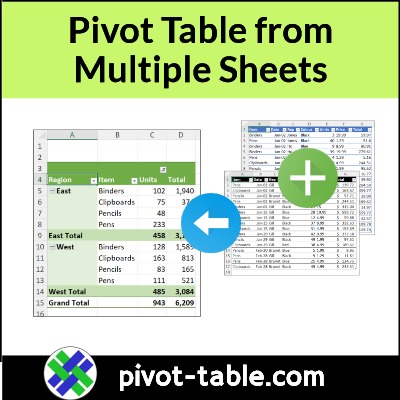
4 Ways to Build Pivot Table from Multiple Sheets
In a perfect world, if you need to make a pivot table, the data is nicely organized in a table, and you can connect to that, quickly and easily.
Unfortunately, as you know, things aren’t always perfect, especially when it comes to data! And sometimes the data is in two or more separate tables, so you need to combine it somehow, before you can build a pivot table..
4 Ways to Combine Data for Pivot Table
There are different ways you can combine data from multiple tables in Excel. For example:
- Power Query
- VSTACK Formula
- Excel Macros
- Pivot Table Wizard
Combine Data Videos
In the sections below, there are a couple of short “Combine Data” videos that I’ve made recently.
- The first video shows how to use the VSTACK function, which is available in Excel 365. It returns multiple ranges in a vertical stack, so it’s easy to combine tables that have identical structures.
- The second video shows how to combine data using the old Pivot Table Wizard. It creates a pivot table with several limitations, but it might do what you need – if you don’t need anything fancy!
For all 4 methods, you can find detailed steps, and sample files, on my Contextures site, on the Pivot Table from Multiple Sheets page .

Video: Create Pivot Table from 2 Tables
Here’s the VSTACK function video, in which I combine the data from tables on 2 separate worksheets. It only takes one cell with a formula, to return all the data from the two tables.
I included the headings for the first table too, because pivot table data needs headings!
Video Timeline
- 00:00 Pivot Table from Multiple Sheets
- 00:20 VSTACK Function
- 00:52 VSTACK Formula
- 01:21 Combined Data
- 01:39 Named Range
- 02:11 Add Pivot Table
Pivot Table Wizard
What if you don’t have Power Query, or the Excel VSTACK function. And you don’t want to use Excel macros?
In that case, you can use the old Pivot Table Wizard to do the job. It’s well hidden in newer versions of Excel, but in the video, I’ll show you how to open it, with an Excel keyboard shortcut.
Video Timeline
- 0:00 Data on 2 Sheets
- 0:24 Open PivotTable Wizard
- 0:50 Select Sheet Ranges
- 1:08 Page Field Settings
- 1:29 Adjust the Pivot Table
- 2:04 Show Sum
- 2:15 Page Field
Get the Sample File
For all 4 methods to combine data, you can find detailed steps, and sample files, on my Contextures site.
Follow this link, to go to the Pivot Table from Multiple Sheets page .
____________________________
4 Ways to Build Pivot Table from Multiple Sheets
____________________________
Move or Lock Pivot Table Field List in Excel
When you create a pivot table, and select a cell in it, a pivot table field list usually appears, at the right side of the Excel window. See how you can adjust that list’s layout, width, and position. Also, see how we moved pivot fields in the olden days – do you remember the PivotTable Wizard?
Continue reading “Move or Lock Pivot Table Field List in Excel”
Quick Trick – Add or Move Excel Pivot Fields
Here’s a quick trick to add or move Excel pivot table fields, just by typing.
Add or Move Pivot Table Fields
Instead of dragging a pivot field into the layout, you can type its name over an existing pivot field label.
- Tip: This is a great shortcut if you like to keep your hands on the keyboard while working in Excel!
Here are the steps to add or move pivot table fields on the worksheet:
- First, change the pivot table to Outline layout or Tabular layout. This trick will not work in Compact layout.
- Next, click on a cell that contains a pivot field name – a cell where you want a different field to appear
- In that cell, type the name of the pivot field that you want to add
- Be careful to type the field name correctly
- If you make a typo, the field won’t be added
- Finally, press Enter, to complete the pivot table layout change
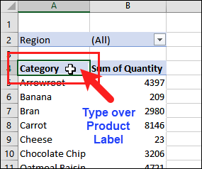
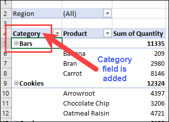
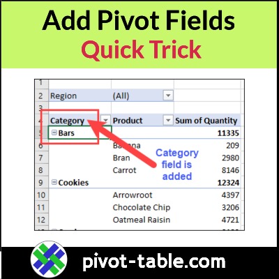
Pivot Field Added
After you press Enter, the pivot table layout changes.
- The field that you typed moves into the active cell.
- The existing fields shift down, and the added field takes its new position.
More Tips for Moving Labels
The first video above shows how to move pivot fields.
You can use a similar trick to move the pivot items in a pivot table.
The short video below shows how to move the Excel pivot items, and you can find written steps on the Move Pivot Table Labels page on my Contextures site.
Get the Sample File
To try the quick trick to add pivot fields, you can use your own pivot table, or download the Move Pivot Labels sample file from my Contextures website.
The zipped Excel file is in xlsx format, and does not contain any macros.
_________________
Quick Trick – Add or Move Excel Pivot Fields
____________________
Show Percent of Group Total – Excel Pivot Table
In an Excel pivot table, you can use Excel’s built-in custom calculations, for a different view of the data.
For example, in the video below, I set up a pivot table to show what % of a company’s monthly sales were Binders. Also, what % of Binder sales was for each colour – red, blue, and black.
Note: You can get the sample Excel file that I used for this video on the Pivot Table Show Values As page, on my Contextures site.
Binder Sales – % By Colour
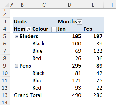
In the screen shot below, the pivot table has 4 fields in the worksheet layout:
- Item and Colour in the Row area
- Month in the Column area
- Sum of Units sold, in the Values area
Following the steps listed in the section below, I used pivot table custom calculations, to show additional sales details:
- the % for each colour‘s sales – Black, Blue and Red
- compared to the item‘s total sales
- in each month – Jan and Feb
Show % of Item Sales
In the pivot table screen shot below, I’ve added a 2nd copy of the Units field to the values area.
- Tip: To add a 2nd copy of a pivot field, drag it from the PivotTable Field list, onto the Values area in the field list
For the 2nd copy of the Units field, I followed the steps below, to change that field’s calculation settings
- Right-click one of the Units value cells
- In the pop-up menu, click Show Values As
- In the next pop-up menu, click % of Parent Row Total
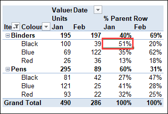
In the pivot table, the second Units field changed, to show:
- the % for each colour‘s sales
- compared to the item‘s total
- in each month.
For example,
- 195 Binders were sold in January
- 51% (100 units) of those January Binders were Black colour
More Pivot Table Info
For more Pivot Table Subtotal tips, videos and examples, visit the following links:
Show Percent of Subtotal in Pivot Table
Pivot Table Show Values As % of Parent Total
Show Percent Of Subtotal In Pivot Table
______________________
30 Years of Excel Pivot Tables-Looking Back
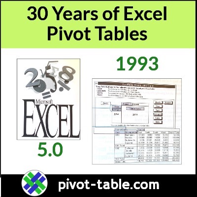
On Saturday, it’s the 38th anniversary of Microsoft Excel, which was released on September 30th, 1985. Eight years later, sometime in 1993, Pivot Tables were added, in Excel 5.0! Happy 30th Anniversary to Excel Pivot Tables.
Continue reading “30 Years of Excel Pivot Tables-Looking Back”
Show All Pivot Table Items To Compare Sales Easily-No Data
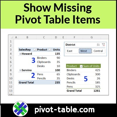
By default, the Pivot Table shows only the items for which there is data. In the example shown in this video, not all colours were sold to each customer. You may wish to see all the items for each customer, even those items with no data.
Continue reading “Show All Pivot Table Items To Compare Sales Easily-No Data”