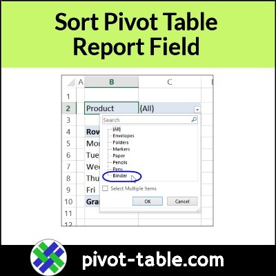
If you have a report filter at the top of your pivot table, do the items in the drop down list ever appear out of order? That happens in my pivot tables occasionally, and there isn’t a quick and easy way to fix the problem!
Video: Sort Pivot Table Report Filters
In the short video below, I show the report filter problem, where the drop down list is not sorted correctly.

After that, I show a workaround that you can use, to get the sorting problem fixed.
There are written steps, and more pivot table sorting tips, on the Pivot Table Sorting Fixes and Tips page, on my Contextures site.
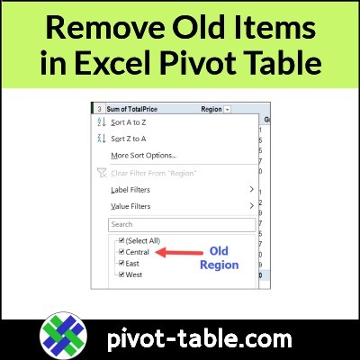
Report Filter Sorting Problem
If you notice that items are out of order in a pivot table report field, you might go to the Data tab on the Excel Ribbon, where the Sort & Filter commands are located.
However, the Sort commands are dimmed out, because you can’t use those in a Report filter field.
Why not? I have no idea!

Report Filter Sort Solution
Fortunately, there’s a workaround that you can use, to sort the report filter items.
It’s not complicated, but it’s a bit annoying that this is the only way to sort things!
To sort the report filter field, follow these steps:
- First, drag the Report field down to the Row area of the pivot table body.
- Next, right-click one of the pivot items in the Report field that you moved to Rows.
- Because the field is in the Rows area, the right-click menu now shows the Sort command
- The Sort commands on the Data tab are available too!
- Click the Sort command, then click one of the sort options – Sort A to Z, or Sort Z to A.
- When the sort is finished, drag the field bad up into the Report Filter area.
NOTE: If you have several Report Filter fields to sort, use the Report Filter sorting macro, on my Contextures site.

Get the Sample File
You can get the Excel sample file, and more pivot table sorting tips, on the Pivot Table Sorting Fixes and Tips page, on my Contextures site.
Also, if you have lots of Report Filter fields to sort, you can save time with the Report Filter sorting macro, on my Contextures site.
__________________________
How to Sort Pivot Table Report Filters

__________________________