Excel Pivot Table: Refresh Automatically With Macros

When you update a pivot table’s source data in Excel, the pivot table does not update automatically. You can set the pivot table to update when the Excel file opens, but that doesn’t help if you’re making changes after the file opens. If you can use macros in your Excel file, you can use an event procedure to force the pivot table to refresh automatically if the source data changes.

Continue reading “Excel Pivot Table: Refresh Automatically With Macros”

Check for Shared Pivot Cache

Last year, I posted Excel VBA code for removing a calculated field from a pivot table.

The code works well if there is only one pivot table based on that pivot cache. However, a couple of comments mentioned that there were problems if multiple pivot tables shared the pivot cache.

Here is a revised version of the code, that checks for other pivot tables using the same pivot cache. If others are found, the macro is cancelled, and a message appears, listing the pivot tables.

pivotcancelmessage 

Remove Calculated Fields for Non-Shared Pivot Cache

If other pivot tables in the workbook share the same cache, the macro is cancelled. A message lists those pivot tables.

Sub RemoveCalculatedFieldsNotShared()
Dim ws As Worksheet
Dim ptA As PivotTable
Dim pt As PivotTable
Dim pf As PivotField
Dim pfNew As PivotField
Dim strSource As String
Dim strFormula As String
Dim iPC As Long
Dim lCache As Long
Dim strPC As String


Set ptA = ActiveSheet.PivotTables(1)
iPC = ptA.PivotCache.Index

For Each ws In ActiveWorkbook.Worksheets
    For Each pt In ws.PivotTables
        If pt.PivotCache.Index = iPC Then
            lCache = lCache + 1
            strPC = strPC & ws.Name & "     " _
                & pt.TableRange2.Address _
                & vbCrLf
        End If
    Next pt
Next ws

If lCache > 1 Then
    MsgBox "Cancelled" _
        & vbCrLf & vbCrLf _
        & lCache & " pivot tables share this pivot cache: " _
        & vbCrLf & vbCrLf _
        & strPC
    GoTo exitHandler
Else
    For Each pf In ptA.CalculatedFields
        strSource = pf.SourceName
        strFormula = pf.Formula
        pf.Delete
        Set pfNew = ptA.CalculatedFields.Add(strSource, strFormula)
    Next pf
End If

exitHandler:
    Exit Sub

End Sub

_______________

Quickly Remove Pivot Table Grand Totals

You probably know how easy it is to add or remove the Grand Totals in a pivot table, by using the Ribbon commands.

But keep reading, to see an even quicker way!

Grand Totals on the Ribbon

Yes, it’s easy to change the Grand Total settings on the Ribbon:

  • Select any cell in the pivot table
  • On the Ribbon, under PivotTable Tools, click the Design tab
  • In the Layout group, at the left, click Grand Totals
  • Click one of the options.

GrandTotalRemove01

Quickly Remove Grand Totals

For an even quicker way to remove Grand Totals, follow these steps:

  • In the pivot table, right-click the Grand Total label cell (not the total amounts) – either the Row Grand Total or the Column Grand Total
  • In the popup menu, click Remove Grand Total

GrandTotalRemove02 

That’s it! Unfortunately, there’s no equally quick way to add Grand Totals, but maybe that feature will be in the next version of Excel.

________

Excel Pivot Table for Financial Data

Last week, you saw a technique for changing monthly data into a better layout, when creating an Excel pivot table.

We used a multiple consolidation ranges pivot table to change this 13-column table into a 3-column data source.

pivot source data monthly

Today we’ll look at a different approach to using multi-column data in a pivot table.

Bi-Weekly Data

Thanks to Jim LaBarr, who sent me a sample Excel file, with his solution to creating reports from multi-column financial data.

In his file, Jim has dates in the heading row – not just the month names. Every column has a heading, and there are no blank rows or columns within the data.

pivot source data bi-weekly

NOTE: Usually, Jim would create an Excel Table from this data, but that changes the headings to text. Don’t create an Excel Table if you want to use the technique that Jim is sharing today.

Pivot Table from Bi-Weekly Data

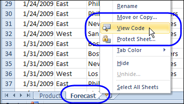
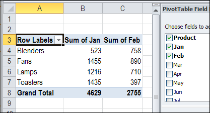
After setting up his bi-weekly financial data, Jim creates a pivot table, using multiple consolidation ranges. This creates a pivot table with 3 fields – Row, Column and Value.

The dates are the Column items, and the descriptions are the Row items.

multiple consolidation ranges

This multiple consolidation ranges pivot table shows a grand total for the columns, because all the dates are in the Column field.

NOTE: If we had created a normal pivot table from the data, each date would be a separate field, and there would be no grand total.

pivot table grand totals

Filter the Pivot Table

After creating the pivot table, Jim filters the Row and Column fields, to focus on specific data. For example, you could filter the Rows to show only the Revenue items (but not the Revenue Total). Then, filter the Columns, to show the December 2010 dates.

The Row and Column grand totals automatically update, to show the totals for the filtered pivot table.

pivot table filtered

Change the Pivot Table Values

When you create a pivot table, the values are summarized by Sum or Count, and shown as simple totals. For a different view of the data, Jim changes the way the Values are shown. In the pivot table shown below, the Values are shown as % of Column.

This is a quick way to see the revenue breakdown, for the two revenue streams. Revenue A produces 60% of the revenue, and 40% is from Revenue B.

pivot table % of column

Grouping the Dates

Because the multiple consolidation ranges pivot table puts the Dates in a single field, Jim is able to group those dates. This gives him even more flexibility in his pivot table reports.

Here, the dates are grouped by year and month, and again, the grand totals are automatically calculated.

pivot table grouped dates

Or, the Column field can be moved to the Row area, to show the dates at the left, in a vertical report.

pivot table vertical

Additional Summary Functions

In another version of his pivot table report, Jim puts 3 copies of the Value field in the Values area.

  • Sum
  • Change
  • % Change

pivot table custom calculations

To show the Change, Jim changes the custom calculation to Difference From. For % Change, Jim uses the % Difference From custom calculation.

pivot table difference from

Create a Pivot Chart

To give a visual overview of the data, Jim create a pivot chart from the multiple consolidation range pivot table. Here, the Years and Months are in the Row area, and the Descriptions are in the Column area, filtered for Total Cost and Total Revenue.

pivot chart finance data

Jim’s Tips for Financial Data Pivot Tables

If your financial data is in many columns, like Jim’s example, here are Jim’s tips for when to use this multiple consolidation ranges techniques, and when to use an Excel Table instead.

  • Use this method to keep multiple columns, with pivot table benefits, like date grouping
  • Use Tables if all you need is Filtering on Rows
  • Use Tables if you need Chart of multiple Rows with no need for time period Grouping
  • For source data with multiple description columns, use the normalization workaround

Download the Sample Financial Data Pivot Table File

To see Jim LaBarr’s sample data, and the pivot tables, you can download his Financial Data Pivot Table sample file. The file is in Excel 2003 format, and zipped.

______________

Friday Fun: Pivot Table Comic

It’s Friday, and the weather has been unbearably hot all week. On top of that, your boss and/or Excel are making you crazy.

If you’re on your last nerve, you can vent your rage in a comic strip, by using Rage Builder. I made this pivot table themed comic, and I’m sure you can do better!

I didn’t upload my comic to the website – I used Snagit to take a screen shot, and save that image file.

ExcelPivotTable_RageComic

________

Fix Pivot Table Source Data For Better Results

When you are setting up your source data for an Excel pivot table, there are a few data layout guidelines that will help you create the best possible pivot table. Get it right, and you won’t have to fix Pivot Table source data later!

Sometimes you get data that isn’t well suited for creating a pivot table, like the example shown below. It has a column for each month, and the sales amounts are spread over those 12 columns.

Continue reading “Fix Pivot Table Source Data For Better Results”

Excel Pivot Table Tweets

twitter_newbird_boxed_blueonwhite It’s interesting to see what people are saying about Excel in Twitter, and I post a few favourite Excel tweets, from my daily reading.

Of course, many of those tweets are about pivot tables, so here, for your Friday entertainment, are some highlights from the past.

Do any of these pivot table tweets sound like you could have posted them?

  • Pivot tables are my favourite part of excel. I’m actually sad enough to have a favourite part.
  • Just discovered the "Show Pages" function in Excel Pivot tables… my world may never be the same again. #dork
  • Pivot tables were originally implemented by Lotus Improv (which was all it did). Yours, the spreadsheet bore 🙂
  • If there was an Olympics for Excel Pivot tables, I would have just done the equivalent of the Double McTwist.
  • You are not the boss of me, Pivot Table. Sorry, I mean Mister Pivot Table.
  • A Pivot Table cannot overlap another Pivot Table – why is this my problem Microsoft?
  • Careful lying about Excel. I got caught in that once. They gave me a test. Stupid pivot tables.
  • Is it me or does excel rarely assume the correct function when i drop data into a pivot table?
  • that’s right ladies, i may not be able to build you a spice rack, but i can sure as hell make you a pivot table. that’s hot, right?
  • Also, if you don’t know how to use pivot tables, you don’t *really* know how to use Excel. There, I said it.
  • OH:"I’m going to write a book about Excel pivot tables. It’s going to be a romance novel."
  • I refuse to help anyone with any system or data unless they know what a excel pivot table is
  • I work with technology every day. Excel pivot tables still baffle me.

Have a great weekend, and may all of your pivot table tweets be happy ones!

__________

Quickly Change Pivot Table Data Functions

It’s easy to change the summary function for one data field in a pivot table. For example, if a field shows the Sum of Units, you can right-click on that field, and change it to Count of Units.

pivottablesummaryfunctions02

However, if you have several data fields in a pivot table, it can take quite a bit of time to change each pivot table summary function manually.

Create a Worksheet List of Functions

To make it easy for yourself, or other people who use the pivot table, to change the functions, you can add a drop down list of functions in a worksheet cell.

PivotFunctionChange02

The list is created with Excel data validation, and Excel VBA code runs when a different function is selected in that cell. The code changes the summary function for all the data fields in the pivot table.

Read the Details

For details on how the code works, you can read the Select Pivot Table Function From Worksheet Drop Down article on the Contextures blog.

Download the Sample File

To test the Summary Function code, you can download the sample file from the Contextures blog link above. The file is in xlsm format, and zipped. Enable macros when you open the file.

________________

Pivot Table Drilldown Formatting

Double-clicking on a number cell in a pivot table creates a new sheet in the workbook, showing the records included in that number. Sometimes the list doesn’t look the way you’d like it to, and the numbers aren’t formatted the way they are in the source data.

For example, the source data might have sales amounts formatted as currency, or dates in a long format.

showdetails12

Unfortunately, those formats aren’t used in the new sheet.

showdetails13

You don’t have much control over the default formatting in the drilldown details list, but here are a couple of things you can do.

Change the Default Table Style

The drilldown details list is formatted as a named Excel Table, in the default style selected in the workbook. If you change the default Table Style, new lists will use the new default style.

To change the default Table Style:
  • Select a cell in any Excel Table in the workbook. If there aren’t any tables, double-click a pivot table data cell, to create one.
  • In the Ribbon’s Design tab, click the More drop down arrow for Table Styles
  • Right-click on the style that you want as the default Table Style
  • Click Set As Default

showdetails07

Now, when you double-click a number cell in the pivot table, the new default style is used.

showdetails08 

Change the Normal Style

If you’re seeing strange number formatting in the drilldown details, such as dates in Currency format, the Normal Style can be adjusted.

When you select a Theme in an Excel workbook, or use the default Theme, it uses specific fonts, colours, and other format settings.

showdetails10

The Normal style is affected by the selected Theme, and you can make further adjustments to the Normal style. The drilldown details list will use the font and number formatting from the Normal style.

To change the Normal style:
  • On the Ribbon’s Home tab, click Cell Styles
  • Right-click on Normal, and click Modify

showdetails09

  • Click the Format button, and change any of the Cell formatting options.
  • Click OK, twice, to close the dialog boxes.

TIP: For number formatting, select General, so dates and numbers will look best. If you select Currency, or another specialized format, all the numbers, including dates, will get that format.

showdetails11

______________

Clean Up Pivot Table Show Details Sheets

When you double-click on the value cell in a pivot table, a new sheet is automatically inserted in the workbook. The new sheet contains a table, listing all the source data records that are summarized in the number that you double-clicked.

showdetails03

Double-clicking the cell is a shortcut to the pivot table Show Details command. You can also right-click on a value cell, and click Show Details.

showdetails02

Show Details, also called DrillDown, is a great feature for digging into the details, but you can end up with lots of extra sheets in your workbook.

However, you don’t usually want to save the sheets, so you manually delete them before you close the file.

Automatically Name the Sheets

With event code on the pivot table’s worksheet, and in the workbook module, you can add a prefix, such as “XShow”, when the Show Detail sheets are created.

showdetails06

That prefix should make the sheets easier to find and delete, before you close the workbook.

Automatically Delete the Sheets

To make the cleanup task even more efficient, you can use programming to show a message when you’re closing the workbook, if there are Show Details sheets in the file.

showdetails04

If you click Yes, all the sheets with the “XShow_” prefix are deleted, and the workbook stays organized. Then, save the tidied up version of the workbook, when prompted.

See the Drilldown Sheet Code

For detailed instructions on adding the drilldown sheet naming and deleting code, visit the Excel Pivot Table Drilldown page on the Contextures website.

Download the Sample Drilldown File

To see how the event code names the sheets, and deletes them when closing, you can download the sample file from my Contextures website, at the link shown above.

________________