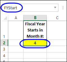
Last week, you saw how to calculate the fiscal year and month, by adding formulas in a pivot table’s source data.
The formulas referred to a named cell – FYStart – where you enter the start month of the fiscal year.
by contextures.com

Last week, you saw how to calculate the fiscal year and month, by adding formulas in a pivot table’s source data.
The formulas referred to a named cell – FYStart – where you enter the start month of the fiscal year.
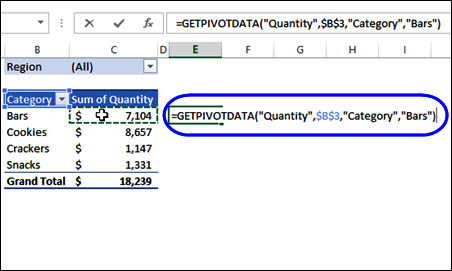
Last week, I did a Pivot Table presentation, and someone asked why you get an absolute reference, if you try to link to a pivot table cell. For example, in the screen shot below, I typed an equal sign in cell E4, then clicked on cell C4, which has the quantity for the Bars category.
That created a GETPIVOTDATA formula, instead of a simple reference to cell C4.
Continue reading “Link to Pivot Table Creates Absolute Reference”
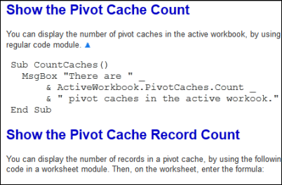
In some of the pivot table articles that I post here, there is sample code that you can use in your own files. Sometimes I show the code sample here, and you can copy and paste it into your workbooks. Other times, I give a link to a file that you can download, and copy the code from that.
If you’re not an Excel programming expert, here are a few tips for copying the Excel VBA programming code to your workbook.
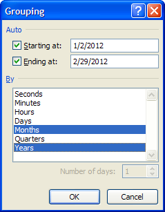
If you’re working with dates in a pivot table, it’s easy to group them by years, months or days – those are options in the Group By dialog box.
However, sometimes you might need a different type of date grouping. In this example, we’d like to group the sales data into 4-week periods, to match our company’s sales calendar. Keep reading to see the steps to set that up, and make sure the period starts on the correct weekday.
A pivot table is a quick and effective way to summarize data, and you can also create a pivot chart, to show a visual summary. And, if you’re summarizing the data by date, you’ll usually need to group the date field, to get a chart that’s easy to read.
Continue reading “Compare Years in Pivot Chart”
When you create a pivot table, Excel applies a default pivot table style. If there are two or more fields in the Row Labels area, you might see dividing lines, below the item headings.
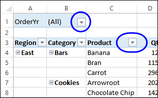
After you set up a pivot table, you might like to prevent people from selecting items in one or more of the heading drop downs.
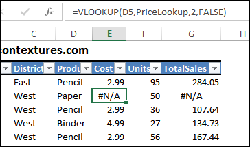
When there are errors in the pivot table source data, you might see errors in the pivot table Values area. In the screen shot below, a VLOOKUP formula in column E has returned an #N/A error, because the product wasn’t found in the lookup table. That also creates an error in column G – Total Sales.
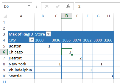
Usually you can only show numbers in a pivot table values area, even if you add a text field there. In the screen shot below, the Max of Region ID is in the Values area.
Instead of the numbers 1, 2 or 3, we’d like to see the name of the region – East, Central or West.