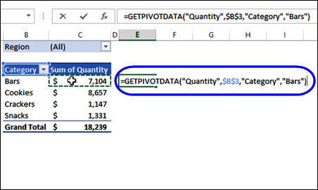
Last week, I did a Pivot Table presentation, and someone asked why you get an absolute reference, if you try to link to a pivot table cell. For example, in the screen shot below, I typed an equal sign in cell E4, then clicked on cell C4, which has the quantity for the Bars category.
That created a GETPIVOTDATA formula, instead of a simple reference to cell C4.

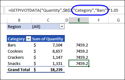
The default GETPIVOTDATA formula acts like an absolute reference – if you copy the formula down the column, it keeps referring to the same cell. In the screen shot below, the formula was created in the row with the Bars category.
When the formula is copied down to the Snacks row, it still refers to the Bars category, and does not give the result that you want in that row.

Turn Off the GETPIVOTDATA Function
The GETPIVOTDATA function is a great tool, for pulling specific data from a pivot table. It’s very fast and efficient, and you can make a few changes to the default formula, to make it flexible. There are GETPIVOTDATA examples on my Contextures web site, that show some of the ways you can tweak the formula, and take advantage of its power.
However, if you just want to create simple links to values in a pivot table, you can turn off this feature.
Here are the steps:
- Select any cell in a pivot table.
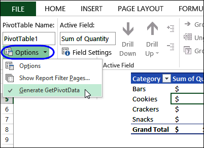
- On the Ribbon, under PivotTable Tools, click the Options tab
NOTE: In Excel 2013, click the Analyze tab - In the PivotTable group, click the drop down arrow for Options
- Click the Generate GetPivotData command, to turn the feature off or on.

Video: Turn Off GETPIVOTDATA Functions
To see the steps for changing the Generate GetPivotData setting in Excel, please watch this short video tutorial.
NOTE: In Excel 2013, the tab name has changed to “Analyze”, instead of “Options”.
Or watch on YouTube: Link to PivotTable Creates GETPIVOTDATA Formula
______________

Great information to know. I do occasionally use a value in a pivot table. Now I know how to change it if I have to. Thanks!!
Thanks JoAnn! Glad it will help you.
I use getpivotdata far more than I do simple links. So in your example I would just put “A4” into the getpivotdata formula in place of “bars” and copy down. Then I don’t have to turn anything off.
Hi,
My pivot table is updated off the other worksheet and it size (the number of rows) is changing every time the source data is changing.
I also calculate another data off pivot table by referencing pivot table sells, similar as in the example “=B4”. But every time the pivot table grows I have to drag down the formula. theoretically I can drag the formula down infinitely, but this is not the best possible solution.
My question. Is it possible to have formulas only in the rows which are exactly the same number as the number of rows in the pivot table? For example, according to the table above, I want column D to be automatically coping formulas, such as “=B4” down to 9 rows only, to “=B13” because the pivot table contains 9 lines of data, but if the pivot table is to change the number of lines to 145, the formulas should be down to the last row of the pivot table, and if the pivot table shrink to 3 lines only, the formula is copied just to “=B6”.
Thank you!!! This has made me crazy. Sometimes the reference/drag worked and sometimes it didn’t and I had no idea why. This will be so useful!
Hello
I am using a standard link to the pivot table rather than getpivotdata. However, when I re-order my pivot table (eg by ascending order) the rows to the side of the pivot table do not follow.
Is there any way to change this without valuing the pivot table?
Thanks
Malcolm
thanks, turn off the option “Generate getPivotData” works for me.