Allow Drag-and-Drop in Excel 2007 Pivot Table

In Excel 2003, you could drag fields from the PivotTable Field List onto the pivot table layout on the worksheet.

In Excel 2007, you can only move the fields to the areas in the PivotTable Field List. In the screen shot below, if you try to drag the Promo field onto the pivot table, the cursor shows an X. The drag-and-drop feature doesn’t work.
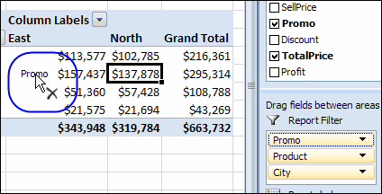
PivotDrag01

Change the Pivot Table Settings

If you’d like to drag the pivot fields onto the worksheet layout, you can change a setting in the pivot table options.

  1. Right-click a cell in the pivot table, and click PivotTable Options.
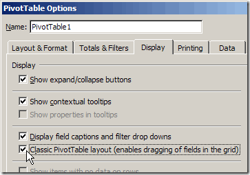
  2. On the Display tab, add a check mark to Classic PivotTable Layout.PivotDrag02
  3. Click OK, to close the PivotTable Options dialog box.

Drag the Pivot Table Fields

After you change the setting, the pivot table on the worksheet shows a blue border around each region.
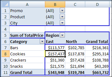
PivotDrag03

You can now drag the pivot fields from the PivotTable Field List onto the worksheet, or drag the fields to a different part of the pivot table.

  1. Point to a field label in the pivot table layout
  2. When the pointer changes to a four-headed arrow, drag the field label to a different area
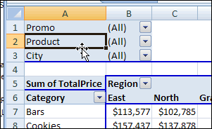
PivotDrag04

You can use the same technique to drag fields into the pivot table layout from the PivotTable Field List, or drag field labels out of the pivot table layout.

Pivot Table in Tablular Form

When you change the setting to Classic PivotTable layout, the pivot table’s report layout automatically changes to Tabular form.

You can use Tabular form, or Outline form, with the Classic PivotTable layout. If you change to Compact form, the blue borders are still visible when the pivot table is active. However, you won’t be able to drag-and-drop the fields.

Video: Classic Layout

In this video, you’ll see the manual steps required to format a pivot table in Classic Style, so you can drag and drop the fields, right on the worksheet. There are several steps in the process:

  • change subtotal setting
  • change report layout of the pivot table
  • change pivot table style
  • change the pivot table display options
  • change setting to clear old items in Pivot Table
  • format each value field as number format
  • sort each row field alphabetically.

Save Time with a Macro: Near the end of the video, you’ll see how much quicker it is to run the recorded macro, to format the pivot able in seconds, instead of minutes. To get that macro, go to the Classic Layout Pivot Table Format Macro page, on my Contextures site.

___________________

Re-create Pivot Table Source Data Table

If you accidentally delete the Excel 2003 worksheet that has the source data for your pivot table, you may be able to use the pivot table’s Drill to Details feature to re-create it.

Extract the Pivot Table Data

To re-create the source data in Excel 2003, follow these steps to use the Drill to Details feature:

  1. Make sure that none of the items in the pivot table fields are hidden. For page fields, (All) should be selected. For row and column fields, (Show All) should be checked. Note: You don’t need to include all the fields in the pivot table before using the Drill to Details feature.
  2. Show the grand totals for rows and columns. If they aren’t visible, right-click a cell in the pivot table, and click Table Options. Check the options Grand totals for rows and Grand totals for columns, then click OK.
  3. Double-click the grand total cell at the bottom right of the pivot table. This should create a new sheet with the related records from the original source data.

Fix the Extracted Data

If the original source data contained formulas, you will have to re-create them, because the Drill to Details feature exports the data only.

The columns in the extracted data will be in the same order as they were in the original source data.

The extracted data will be formatted with Table AutoFormat List 3. You can apply a different AutoFormat, or apply your own formatting.

Note: If you had made changes to the source data and not updated the pivot table, those changes won’t be in the extracted data.

Connect to the Extracted Data

If you rename the sheet that was created during the Drill to Details process, and use the same name as the worksheet that originally held the source data, the pivot table might automatically connect to the new source data table.

If not, you can connect to the re-created source data:

  1. Right-click a cell in the pivot table, and choose PivotTable Wizard.
  2. Click the Back button, and select the new source data table range.
  3. Click Finish.


Pivot Table Error: Excel Field Names Not Valid

Usually, things go smoothly when you when you try to create a pivot table. However, occasionally you might see a pivot table error, Excel Field Names not Valid, if you try to build a new pivot table, or refresh an existing pivot table.

Updated Jan. 1, 2019 – macro to help with troubleshooting the pivot table error

Continue reading “Pivot Table Error: Excel Field Names Not Valid”

Create Two Pivot Tables on Excel Worksheet

In a comment on this blog, someone asked how to create two pivot tables on the same Excel worksheet.

NOTE: See the updated version of this Two Pivot Tables article, from July 2020.

Shown below is a worksheet named Pivot_Reports, with a pivot table on it, based on the data on the Sales_East sheet.

TwoPT01

We’ll add another pivot table to the Pivot_Reports sheet, based on data on the Sales_North sheet.

Add the Second Pivot Table

  • Select the Sales_North sheet, and select a cell in the data table.
  • On the Ribbon, click the Insert tab
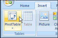
  • In the Tables group, click PivotTable (click the top half of the PivotTable command).

RibbonInsertPT

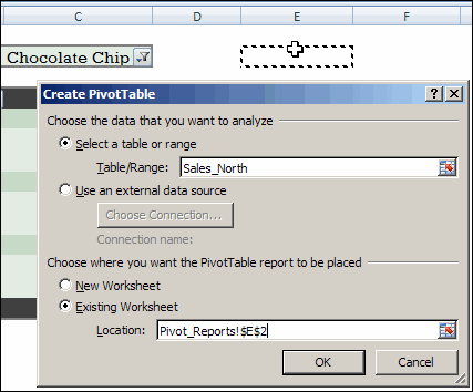
  • In the Create PivotTable dialog box, at the top, leave the default selection of Select a Table or Range, where the Sales_North table shows.
  • In the lower section, click Existing Worksheet.
  • Click in the Location box, then click on the sheet tab for the Pivot_Reports sheet.
  • Click on the cell where the second pivot table should start.

TwoPT02

  • Click OK to create the new pivot table.
  • Add the fields that you’d like in the new pivot table.

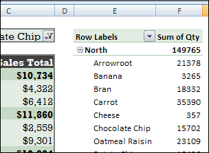
The second pivot table is added to the Pivot_Reports worksheet.

TwoPT03

Prevent Pivot Table Overlap

When you have two or more pivot tables on the same worksheet, be careful to prevent them from overlapping.

PTOverlap

Before you add new fields to the pivot table on the left, you might have to add blank columns between the pivot tables. Or, if one pivot table is above the other, add blank rows between them.

If the pivot tables will change frequently, adding and removing fields, it may be better to keep the pivot tables on separate sheet.

This short video shows pivot table refresh problems, and how to avoid them. For detailed written notes, go to the Pivot Table Errors page on my Contextures site.

Related Articles

Create a Pivot Table In Excel

Create Two Pivot Tables On Excel Worksheet

____________

Hide Error Values in Pivot Table

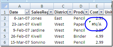
Sometimes there are errors in the source data on which a pivot table is based.

ErrorWksht

In most cases, I like to see the errors on the worksheet, so that problems are easy to spot. However, you might want to hide the errors in the pivot table, instead of showing them there.

By default, error values are displayed in a pivot table. However, by changing the PivotTable Options, you can hide the errors so blank cells appear instead of the errors:

  • Right-click a cell in the pivot table
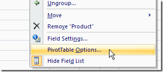
  • In the context menu, click PivotTable Options.

PTOptions

  • In the PivotTable Options dialog box, click the Layout & Format tab.
  • In the Format section, add a check mark to For Error Values, Show.PTErrorVal
  • Leave the text box blank, and the errors will be replaced with blank cells. Note: You could type other characters, such as a hyphen, in the text box, to replace the error values with that character.
  • Click OK to close the dialog box.

Note: This setting only affects cells in the Values area of the pivot table. If error values appear in the Row Labels, Column Labels, or Report Filter area, they won’t be replaced.

_____________________

Create an Excel Table in Excel 2007

An Excel Table is a new feature in Excel 2007, similar to the List feature in Excel 2003. An Excel Table makes it easy for you to sort, filter, and review your data, whether it’s a few rows and columns, or thousands.

You can also use an Excel Table as the source for a Pivot Table, and new data will automatically be included in the Pivot Table source.

Arrange Your Data

Prepare your data before creating an Excel Table:

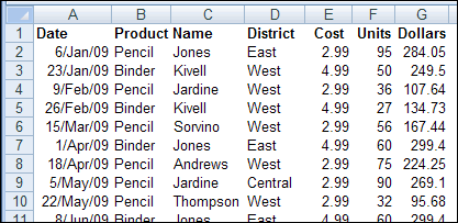
  • Enter your data on a worksheet, in rows and columns, with headings in the first row.
  • Remove any blank rows or columns within the data
  • Leave at least one blank row and one blank column between your data, and any other data on the worksheet. Ideally, keep your data on a separate sheet.

Create the Excel Table

To create an Excel Table:

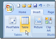
  • Select a cell in your data, and on the Ribbon, click the Insert tab.
  • In the Tables group, click the Table command.
  • RibbonInsertTable
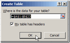
  • In the Create Table dialog box, the range for your data should automatically appear, and the My table has headers option is checked. Click OK to accept these settings.
  • CreateTableOK

Explore the Excel Table Features

After you have created an Excel Table, you can test some of its useful features:

  • Sort Data — Click drop down arrow in the heading cells, and click to sort data in ascending or descending order.
  • Quick Filters — Click drop down arrow in the heading cells, and check or uncheck items to show or hide.
  • Visible Headings – If headings in row 1 are no longer visible, column letters are replaced by Excel Table headings.
  • New data automatically included–Add data at the end of an Excel table, and the table automatically expands to include it.
  • Table Name –An Excel table is automatically named, e.g. Table1, when it is created. You can refer to this name when creating a pivot table. You can also change the name to something better, such as SalesData.

Excel Table Tutorial Video

If you’re working with lists of data in Excel 2007, be sure to use the new Excel Table feature, to make it easier to manage your data.

To see a quick demonstration of creating an Excel Table, and testing a few features, please watch this short video tutorial.

____________

Deleting the Entire Pivot Table

To remove a pivot table from an Excel workbook, you can delete the worksheet that the pivot table is one.

Occasionally, you might want to remove a pivot table, but you can’t just delete the worksheet because it contains other data. To remove a pivot table, and leave the other items on the sheet untouched, you can clear the cells.

Clear the pivot table cells

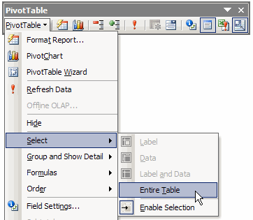
1. Select a cell in the pivot table

PivotSelectTable

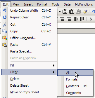
2. On the menu bar, click Edit|Clear|All.

3. On the PivotTable toolbar, click PivotTable|Select|Entire Table

This will remove the pivot table, and all its formatting, from the worksheet.

Note: After deleting the pivot table, you might temporarily see drop down arrows where the pivot fields were located, but these should disappear when you activate another cell.

___________________________

For more information on pivot tables, see the Pivot Table Topics on my Contextures web site.

___________________________