Create and Filter Two Pivot Tables on Excel Sheet

Usually, it’s best to set up your Excel file with one pivot table per sheet, so you don’t have to worry about them overlapping. However, if you need to see them side by side, here’s how you can create and filter two pivot tables on an Excel sheet, based on the same source data.

Create First Pivot Table

Watch this video, to see the steps for quickly creating a pivot table in Excel, using the Recommended PivotTables feature.

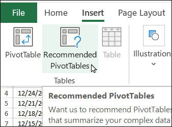
To find the the Recommended PivotTables feature, go to the Insert tab on the Excel Ribbon. For the detailed written steps, go to the Create an Excel Pivot Table page on my Contextures website.

TIP: On that page, you can also download the Region Sales sample file that was used in this example

Prepare for the Second Pivot Table

Before you create the second pivot table on the same sheet, do these preparation steps:

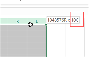
To the right of the first pivot table, select about 10 columns

TIP: As you drag across the column buttons, to select the columns, the tool tip shows how many columns have been selected.

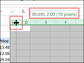
Reduce the column width of the selected columns, to about 2.00 (19 pixels)

This creates space between the two pivot tables, to prevent accidental overlapping, if you refresh them.

TIP: If the columns are hidden, you won’t notice if the first pivot table expands slightly, to fill one or more of the “spacer” columns. It’s better to make them narrow, so you can see any problems immediately.

Create Second Pivot Table

The easiest way to create a second pivot table, based on the same source data, is to copy and paste the first pivot table.

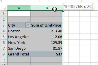
First, select all the columns where the first pivot table is located

Next, press Ctrl+C to copy the selected
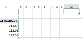
Then, select the cell in row 1, in the column where you want to paste the new pivot table. In this screen shot, columns C to L are narrow, and cell M1 is selected.

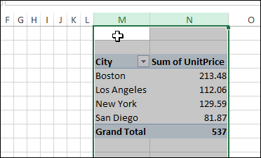
Press Ctrl+V to paste the pivot table columns in the new location

Then, to complete the second pivot table, add or remove fields, or change the layout as needed.

Refresh Problems With 2 Pivot Tables

When you have two pivot tables on an Excel sheet, you might see error messages occasionally, when you refresh the pivot tables.

This short video shows the problems, and how to avoid them. For detailed written notes, go to the Pivot Table Errors page on my Contextures site.

Slicer to Filter Both Pivot Tables

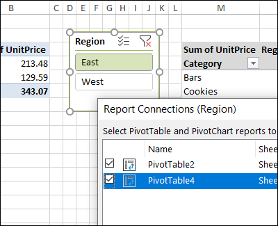
The final step in setting up the two pivot tables is to add a Slicer. Because both pivot tables are based on the same source data, they can both be connected to the same Slicer.

In this video, you’ll see the easy steps to add a Slicer, based on the first pivot table. Next, see how to connect the second pivot table to the same Slicer. There are written instructions on the Contextures Pivot Table Slicers page.

Get the Sample File

To download the Region Sales sample file, go to the Create an Excel Pivot Table page on my Contextures website. The zipped file is in xlsx format, and does not contain macros.

_______________________