Click a pivot table Slicer, to quickly show and hide groups of values. This value group slicer technique saves time and space, when there are lots of numeric fields in your source data table.
Value Group Slicer Demo
This animated gif shows how this value group Slicer technique works.
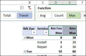
- Click a button on the Group Slicer, to quickly show those fields in the pivot table.
- Click the Function slicer to set the function and headings.
Source Data Table
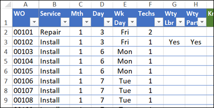
In this example, there’s a table with work order data, and a pivot table based on that data. You can use this technique in your own workbook, using other types of data.
The work order table has several columns with descriptive data, and those would be used in the Row, Column and Filter areas of a pivot table.
Fields for Values Area
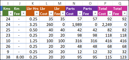
The work orders table also has lots of columns with numeric data. Those are the fields that we’d put in the pivot table’s Values area.
There are 4 different groups of numeric data, and I’ve colour coded the column headings, to make the groups easier to identify.
- Travel — Kms, Km Fee
- Labour — Lbr Hrs, Lbr Cost, Lbr Fee
- Parts — Parts Cost, Parts Fee
- Total — Total Cost, Total Fee
Pivot Table Value Fields
If you put all those numeric fields into the pivot table at once, you’ll end up with a crowded report, that’s hard to read.
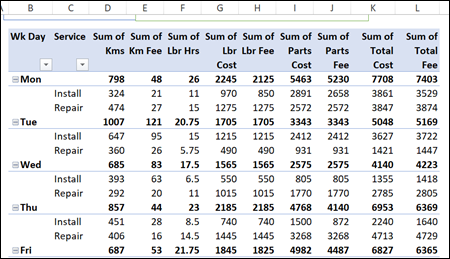
You could manually add and remove the Value fields, a few at a time, to reduce the clutter. However, that might get annoying, before too long!
Instead, this example uses a Slicer to add Value groups, quickly and easily. There’s also a Slicer to change the function that each value field uses.
How It Works
All the details of how this works are on the Value Group Slicers page on my Contextures site. But here’s a quick overview.
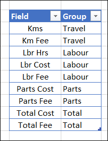
The key to the Value groups is a named table, where the numeric fields are all listed. In the next column, each field is assigned to one of the value groups.
NOTE: When you adapt this technique for your own data, list all the your numeric fields, and create group names that suit your data.
Pivot Table and Slicer
The workbook has a pivot table that’s based on the field list, with the Group field in the pivot table’s Filter area.
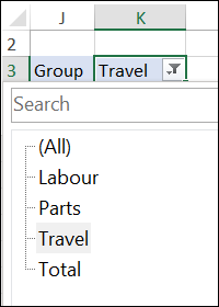
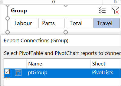
There’s a Slicer connected to that pivot table, and it’s on the worksheet with the main pivot table.
Get the Fields
To see which fields belong to the selected group, there’s a dynamic array formula:
- =SORT(FILTER(tblFields[Field], tblFields[Group]=K3))
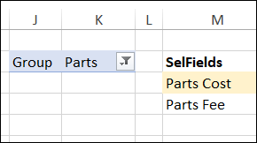
The formula is in cell M4, and it spills into the cells below. The list resizes automatically to show all of the fields for the selected group.
Value Groups Macro
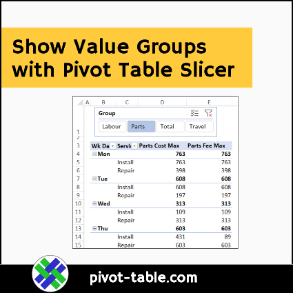
When you click a Group button on the pivot table Slicer:
- pivot table filter updates, to show the selected group
- field list in column M updates automatically
- macro runs automatically, to show the fields from the selected group
The complete macro code is on my Contextures site, and in the sample file.
Get the Sample File
To get the sample file, and to see the details on how this technique works, go to the Value Group Slicers page on my Contextures site.
The file is zipped, and is in xlsm format. The file contains macros which run when the slicers are clicked. Be sure to enable macros when you open the workbook, if you want to test the Slicers.
_____________________
Value Group Slicer for Excel Pivot Table
_____________________