Pivot Table from Visible Rows in List

When you create a pivot table in Excel, it includes all the source data, even if some rows were hidden by filtering. However, if you’re using a version of Excel that has the new Spill (dynamic) functions, you can try this technique, to create a pivot table from filtered list visible rows only

New Spill Functions

This technique uses new features in Excel, that are found in Excel for Office 365. Try these steps, to see if you have the new functions:

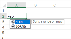
Select a blank cell, then type: =SO
If the screen tip shows SORT and SORTBY, you have the new functions.

Best for Small Data

In this example, there are only 100 rows of data in the source table. I didn’t notice any slow calculation problems while working on this file.

However, if your pivot table source data has a large number of records, this visible data technique could slow down your workbook

Named Excel Table

In this example, the source data for the pivot table is a formatted Excel table named Sales_Data.

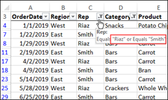
There are 100 records in the table, and two of the columns have filters applied:

Rep – only Smith and Riaz are showing
Category – the Cookies category is hidden

Make a Pivot Table

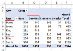
Even though some of the rows are hidden by filters, when you create a pivot table from the Sales_Data table, it includes all 100 records, not just the visible row records.

All the sales rep names are listed, not just Smith and Riaz
All the categories are included.

Pivot From Filtered List

There isn’t a built-in way to use just the visible data, so you can try this workaround technique instead.

Here’s an overview of the steps for the workaround:

Add a column in the source table, with a formula to mark visible rows
On another sheet, get the source data headings
Use a Spill function to pull visible rows from the Sales_Data table
Create a dynamic named range, based on pulled data and headings
Create a pivot table based on the dynamic named range

1. Mark Visible Rows

First, add a new column in the Sales_Data table, with the heading Vis

Then, in cell J4, enter this formula that uses the SUBTOTAL function:

=SUBTOTAL(2,[@Orders])
Press Enter

The formula is automatically copied down to all the cells in the Vis column, even the hidden rows

How It Works

The SUBTOTAL function ignores values that are hidden by a filter, so for non-visible rows, the result in column J is zero.

For example:

row 18 is visible, so it returns a 1
row 19, is hidden by the filter, so it returns a zero

Later, we’ll be able to get the visible rows, because they’ll have a 1 in the Vis column.

New Source Data

Next, you’ll start a new source list for the pivot table

Insert a new worksheet, and name it, DataFiltered

To use this as a pivot table source, the data needs headings. Follow these steps to use the headings from the Sales_Data table.

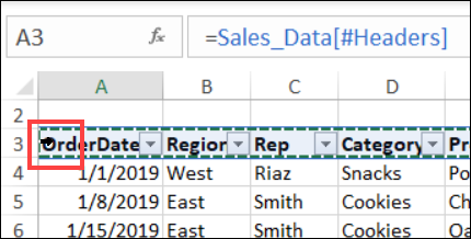
In cell A1 on the new sheet, type an equal sign
Go to the FoodSales sheet, and click at the left edge of cell A3, to select all the heading cells
Press Enter, to complete the formula

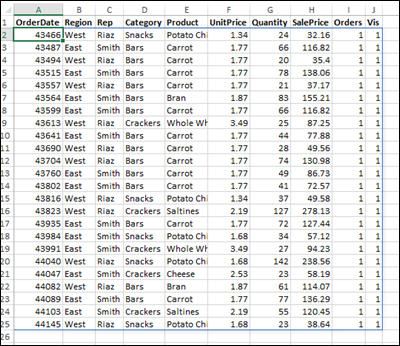
The headings will automatically “spill” across the columns on the DataFiltered sheet.

Get the Filtered Data

Next, we’ll use a new Excel function — FILTER — to pull the visible rows from the Sales_Data table

Select cell A2, and enter this formula:

=FILTER(Sales_Data,Sales_Data[Vis]=1

Spill Formula

Even though you only entered the formula in cell A2, the formula results spill down and across, in as many cells as needed.

There is a thin blue border around the dynamic array

Cells in the Dynamic Array

If you click in any cell in the dynamic array, other than cell A2,

you can see the formula in light grey font in the formula bar
you can’t make any changes to the formula

If you select cell A2, where the formula was entered, you can edit the formula, as usual

Create a Dynamic Named Range

Next, we’ll create a dynamic named range to use as the pivot table’s source data. This range will include the heading cells, and the filtered data.

To refer to a dynamic array, use the array’s starting cell, followed by the spill operator – #. For example: DataFiltered!$A$2#

Follow these steps to set up the named range:

On the Excel Ribbon, click the Formulas tab, then click Define Name
For the Name, type: PivotUse
Leave the Scope as Workbook
In the Refers to box, enter this formula:
- =DataFiltered!$A$1#:DataFiltered!$A$2#
Click OK, to complete the name

Create the Pivot Table

The final step is to create a pivot table, based on the dynamic named range.

Insert a new sheet, and name it PivotVis
Select any cell on the new sheet
On the Excel Ribbon, click the Insert tab
Click the Pivot Table command
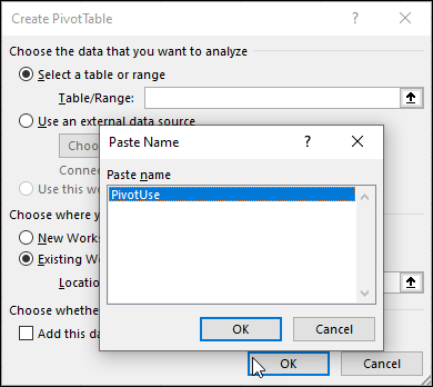
In the Create PivotTable dialog box, click in the Table/Range box, and press the F3 key on your keyboard
In the Paste Name list, click on PivotUse, and click OK
For the location, choose the PivotVis sheet
Click OK to create the pivot table.

Add Fields to the Pivot Table

Next, use the PivotTable Field List to add the fields that you want to show in the pivot table.

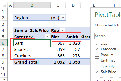
If you include the Rep and Category fields, you’ll see that they only include the items from the visible rows in the Sales_Data table.

Change the Sales_Data Filters

If you change the filters in the Sales_Data table, be sure to refresh the pivot table after you’ve finished making the changes.

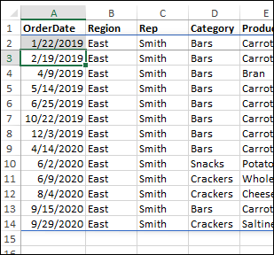
For example, filter the data so it only shows sales in the East region.

The dynamic array updates automatically, and now there are only 14 rows on that sheet.

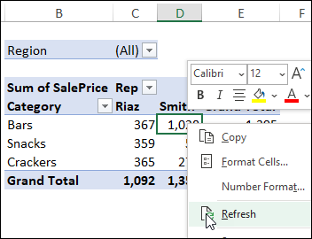
However, pivot tables don’t refresh automatically, so you can do that step manually.

Right-click on the pivot table, and click Refresh.

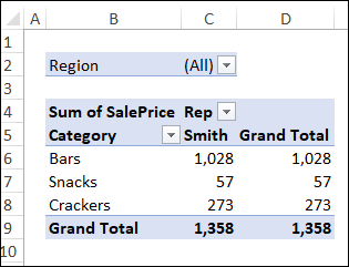
After the refresh, only the East region records are showing. Riaz didn’t make any sales in that region, so Smith is the only rep in the filtered data, and in the refreshed pivot table.

Get the Sample File

To see how the pivot table from filtered list visible rows technique works, go to the Pivot Table Source Data page on my Contextures site.

In the Download section, get the Filtered Source Data sample file. The zipped file is in xlsx format, and does not contain any macros.

____________________________