Change All Pivot Charts with Single Cell Filter

If you have several pivot charts on an Excel dashboard, and space is limited, here’s a way to change all pivot charts with a single filter cell. When you select a different date from the drop down in that cell, all the pivot charts are automatically updated. There are NO macros for this technique, just Slicers, that are stored on a different sheet.

Single Cell Filter

If there’s lots of room on your dashboard sheet, you could put Pivot Table Slicers there, and use those to update the pivot charts. If dashboard space is limited, use this single cell filter technique instead.

Thanks to AlexJ, who shared this technique for using a single cell filter, to update multiple pivot tables and pivot charts. The pivot tables and Slicers are stored on a different worksheet, so they don’t take up room on the dashboard.

This video shows how to set things up, and then filter all the pivot charts with a single cell filter. There are written details below the video.

Dashboard with 2 Filter Cells

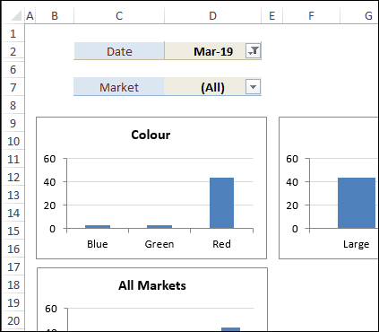
Here is a screen shot of the dashboard, with two single cell filters at the top of the sheet.  One filter is for the date, and the other filter is for the Market areas (East, West, North and South).

One or More Slicers

In the file that AlexJ sent to me, he had one Slicer set up, to filter the Date field in all the pivot charts.

The technique works well with more than one filter too, and I’ve added a Market Slicer in the sample file that you can download.

Note – If you’re using more than one master filter, AlexJ warns us to leave a few blank rows between them. Otherwise, you’ll see a message that pivot tables can’t overlap one another.

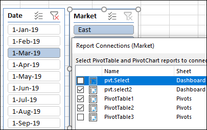
Choose Connections

You don’t need to connect all the pivot tables to all the Slicers though. As you can see in the screen shot below, the third chart is not connected to the Market filter – it always shows the results for all markets.

However, the pivot tables are all connected to the same Date slicer, so when you select a date, all the pivot charts change.

Set Up

There are only a few steps to set up this single cell filter technique.

1. Create Pivot Tables

• First, create a pivot table, based on your data in Excel. There are details on my Contextures site, if you’d like to see how to do that.
• Next, copy the first pivot table, and paste another copy onto the worksheet, leaving several blank columns between them.
• Paste more copies of the pivot table, if needed – one for each pivot chart that you want to create.
• Set up the fields in each pivot table, based on what you want to show in each pivot chart
• Add one more pivot table, with just the field that will be used as a filter – the Date field, in this example. That field goes into the Filter area in the pivot table. Don’t add any fields to the Row, Column or Values areas
• (optional) Set up another pivot table to use for filtering, and put a different field in the Filter area – Market, in this example

2. Create Pivot Charts

• Next, create a pivot chart based on each of your pivot tables. There are details on my Contextures site, if you’d like to see the steps.
• Then, move all the pivot charts to the dashboard sheet

3. Insert a Slicer

• Next, select a cell in any one of the pivot tables, and insert a Pivot Table Slicer.
• Connect all of the pivot tables to that Slicer
• (optional) Add another Slicer, and connect it to some or all of the pivot tables

4. Move the Filter Cells

• Finally, cut the filter cells from the pivot table sheet (the small pivot table with 1 field only)
• Paste that pivot table at the top of the Dashboard sheet, to use as a filter for all the pivot charts.
• If you created other pivot tables to use as filters, move those to the Dashboard sheet too.

Download the Sample File

To see how this technique works, go to my Contextures website, and download the completed sample file. On the Sample Excel Files page, go to the Pivot Tables section, and look for PT0031 – Change All Pivot Charts With One Filter.

____________________

Change All Pivot Charts with Single Filter