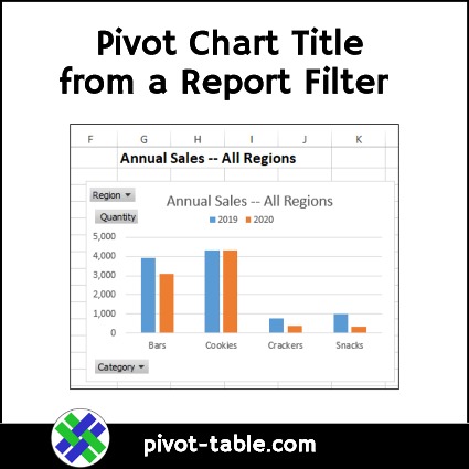
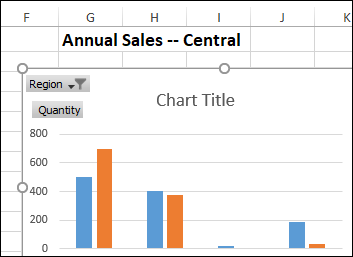
Get Pivot Chart Title from a Report Filter Cell

Instead of typing a pivot chart title, which never changes, use this method to create a dynamic heading. See how to create a formula on a worksheet, then link to that cell, to create a pivot chart title from a report filter cell.

Pivot Table With Report Filter

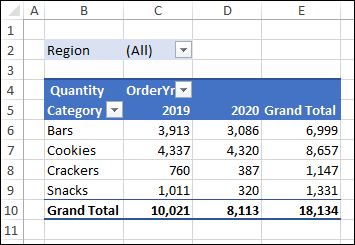
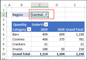
In this example, there is a pivot table with one field, Region, in the Report Filter area. The pivot table shows quantity sold over 2 years, in each food category.

You can select a region name from the drop down list, and the pivot table shows the sales in that region.

NOTE: To follow along with this tutorial, go to the Pivot Chart page on my Contextures blog, and download the sample file. The sample file contains the completed formula and pivot chart. You can delete those, and build your own.

Pivot Chart Title Video

To see the steps for creating a dynamic Pivot Chart title, watch this video. The video timeline, and written instructions, are below the video.

Video Timeline

00:00 Intro
00:19 Add a Pivot Chart
01:14 Add a Chart Title
01:57 Region Filter
03:01 Create a Formula
03:22 Formula Rules
04:02 Start the Formula
06:52 Link Title to Formula Cell
07:51 Get the Sample File

Create a Pivot Chart

To create a pivot chart from the food sales pivot table, follow these steps:

Select a cell in the pivot table
On the Excel Ribbon, click the Insert tab
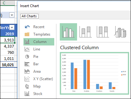
In the Charts group, click Recommended Charts
Click OK, to accept the recommended chart layout – a Clustered Column chart.

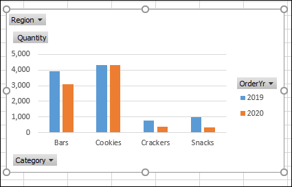
A pivot chart is added to the worksheet, showing the 2 years of data.

Add a Chart Title

There’s no title on the chart, so follow these steps to add a title:

With the pivot chart selected, click the Design tab on the Excel Ribbon
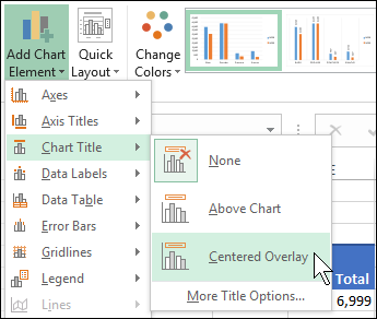
At the left, click Add Chart Element
Then, click Chart Title, and click the “Centered Overlay” option – that adds a title, without making the plot area smaller

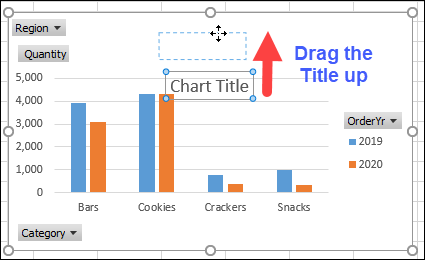
A generic title is added to the pivot chart, with the text “Chart Title”.

Drag the chart title up, to position it in the blank space above the plot area.

Pivot Table Region Filter

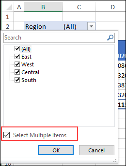
There are four regions in the food sales data – East, West, Central and South. The “Select Multiple Items” option is turned on, so you can select one or more of the regions.

Based on the selection in the Report Filter, cell C2 will show one of these results:

(All) – if no filter has been applied yet, or if (All) was selected
Region Name – if a single Region was selected
(Multiple Items) – if 2 or more Regions were selected, but not all Regions

Chart Title Text Options

Instead of typing a new chart title in the Title box, we’ll create a chart title formula, in a cell on the worksheet. That will help us build a dynamic title, to show details on what was selected in the Region filter.

We want the chart title to say “Annual Sales — “, followed by information from the Report Filter cell, C2.

Based on the value in cell C2, this text should appear in the pivot chart title:

(All) – show “All Regions”
Region Name – show the selected Region name
(Multiple Items) – show “Multiple Regions”

Create a Chart Title Formula

To check for those 3 Report Filter options, we’ll build a nested IF formula. The formula can’t go directly into the chart title, so we’ll build it on the worksheet, then link to the formula cell.

Enter the following formula in cell G2 (I’ve added line breaks, so it’s easier to read):

=”Annual Sales — ” &
IF(C2=”(All)”,”All Regions”,
IF(C2=”(Multiple Items)”,”Multiple Regions”,C2))

That formula starts with the text string =”Annual Sales — ”

Then, if cell C2 contains “(All)”, the result ends with “All Regions”
Or, if cell C2 contains “(Multiple Items)”, the result ends with “Multiple Regions”
Otherwise, show the selected Region name, from cell C2

Format and Move

Next, you can format the formula cell to make it bold font, and a bigger size. Then, move the chart up, so it is just below the formula cell.

Or, if you don’t want to see the worksheet formula, move the chart up to cover cell G2

Link Chart Title to Formula Cell

The final step is to link the pivot chart title to the formula cell. Follow these steps to do that:

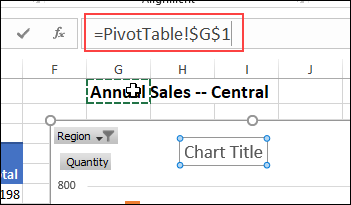
Click on the chart’s title, to select it. Don’t click inside the chart title, just the border. If you see the cursor flashing in the text, click on the title border, to exit the text editor.

Next, click in the Formula bar, and type an Equal Sign (=)
Click on cell G1, which contains the pivot chart title formula

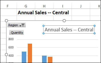
Next, press Enter, to complete the link formula in the chart title

The pivot chart title now shows the result of the formula in cell G1.

Test the Pivot Chart Title

To make sure that the formula is working correctly, make a few changes with the Region Report Filter:

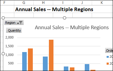
First, select an additional Region, so that cell C2 shows “(Multiple Items)”. The chart title should change to “Annual Sales – Multiple Regions”.
If necessary, move the Chart Title so it is centred above the plot area

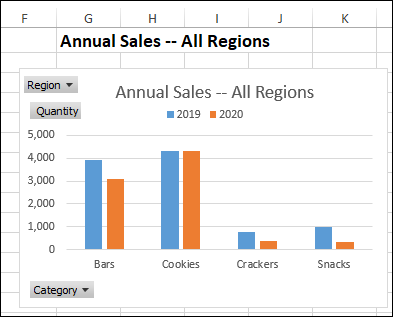
Next, select (All) in the Region Report Filter, to show data for all the regions. The chart title should change to “Annual Sales – All Regions”.

Final Touches

To make the pivot chart look even better, you can add a couple of final touches:

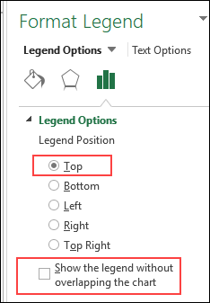
Right-click the Legend, and click Format Legend
In the Format Legend Task Pane, select Top as the position
Remove the check mark for the setting “Show the legend without overlapping the chart”
Close the Format Legend Task Pane

Then, follow these steps to hide some or all of the field buttons:

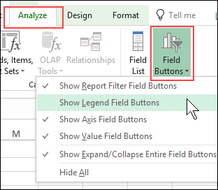
On the Excel Ribbon, click the Analyze tab
At the far right, click the arrow for Field Buttons
Click on “Show Legend Field Buttons” to toggle that setting
- OR, to hide all the field buttons, click on “Hide All”, at the bottom of the list (Note: You’ll need to adjust the plot area size, etc., if you turn off all the buttons)

Then, move the Chart Title and Legend, if necessary, so they fit in the blank space above the plot area.

Download the Sample File

To follow along with this tutorial, go to the Pivot Chart page on my Contextures blog, and download the sample file. The sample file contains the completed formula and pivot chart. You can delete those, and build your own.

______________________