How to Use Different Number Format in Excel Pivot Chart

When you create a new pivot chart in Excel, its number formatting is copied from the pivot table that it’s based on. See how to change the pivot chart number formatting, without affecting the pivot table’s number formatting. If you have several pivot charts to change, use a macro to make the job easier.

Video: Pivot Chart Number Format

This short video shows how to change the number format for the pivot chart only, or change the number format for both the pivot chart and the pivot table. There are written steps below the video.

Pivot Chart Default Format

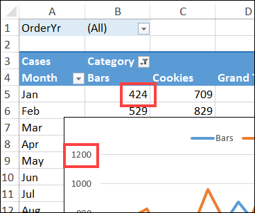
Here is a simple pivot chart, with its pivot table in the background. It’s showing the number of cases sold per month.

In both the pivot table, and the pivot chart, the numbers are in General format, with no separators or decimal places.

Change Pivot Chart Number Format

To use a different number format in the pivot chart, follow these steps. This change will not affect the pivot table – its number formatting will stay the same.

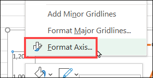
First, in the pivot chart, right-click a number in the axis, and then click Format Axis

Next, in the Format Axis pane, go to the Axis Options tab

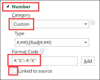
Click the arrow to the left of Number, to see the options
From the Category drop down, select Custom.
This automatically removes the check mark from Linked to Source, and disconnects the axis labels from the formatting in the pivot table.

Add Your New Format

Next, in the Format Code box,

Type a code for the number formatting that you want to use, such as: #,”K”;-#,”K”
Or, select a format from the Type drop down
Then, if you created a new format, click Add, to create the custom number format code.

See the New Format

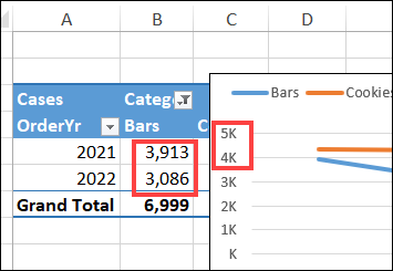
Close the Format Axis pane, and only the pivot chart number format has changed.

The pivot table numbers are still in the previous format

Change Axis Units Setting

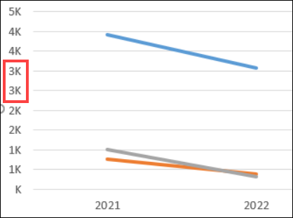
If you see duplicate numbers in the pivot chart axis, you might need to adjust the Axis Units too.

Here’s how to change the Axis Units setting:

In the Format Axis pane, to to the Axis Options tab
Click the arrow to the left of Axis Options, to see the settings.
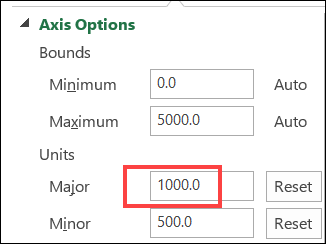
In the Units section, enter a number for Major that works with your number formatting.
For this example, I entered 1000, because the pivot chart axis shows the values in thousands.

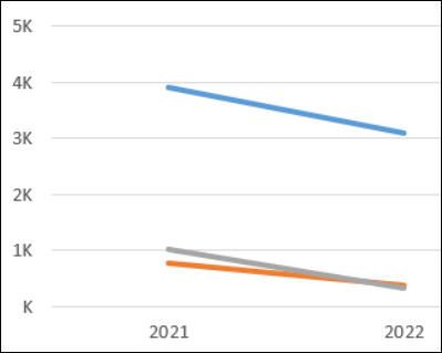
That removes the duplicates from the pivot chart axis.

More Custom Number Format Examples

Here are a few more custom number formats you could use in your pivot chart.

Code	Format
#.00	2 decimals
#,	Thousands
#.0,	Thousands, 1 decimal
#.00,,	Millions, 2 decimals

To see even more number format code examples, go to the Number Format Codes page on the Microsoft site.

Use a Number Format Macro

If you have lots of pivot tables to change, use this macro to make the job easier. You can change the number format in the code’s strFmt variable, to match the formatting that you need.

For details on how to use the macro, go to the Pivot Chart Number Formatting page. You can also download the sample workbook there. It has this pivot chart formatting macro, and sample pivot charts for testing.

Sub FormatChartNums()
Dim ws As Worksheet
Dim pc As ChartObject
Dim strFmt As String
On Error Resume Next
strFmt = "#,##0"

For Each Ws In ActiveWorkbook.Worksheets
  For Each PC In ws.ChartObjects
    With pc.Chart
      'test for pivot charts
      If Not .PivotLayout Is Nothing Then
        .Axes(xlValue).TickLabels _
          .NumberFormat = strFmt
      End If
    End With
  Next PC
Next Ws

End Sub

_______________