If you’re building a formula, and you click on a pivot table value, Excel might insert a GetPivotData formula, instead of a cell reference. Here’s how you can stop that annoying problem from happening.
Pivot Table Limitations
Pivot tables are powerful, but they can’t do everything. So, sometimes you add formulas beside a pivot table, to overcome those limitations.
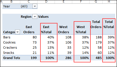
For example, you might want to see percentages for your row totals, as well as the numbers. To do that, you could add a second copy of the number field, and set it to show % of Column Total.

However, you can’t just do that for the Grand Total – it shows the percentages for other columns too. That can clutter up a pivot table, and makes it hard to see the other data.
Formulas Outside the Pivot Table
So, instead of adding another copy of a number field, you might decide to put formulas at the right side of the pivot table, and calculate the percentages there.
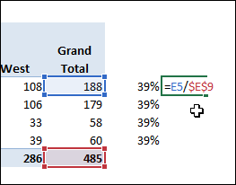
In this example, the formula for the first percentage should be: =E5/$E$9
That will let us divide the total in each row, by the grand total in E9.
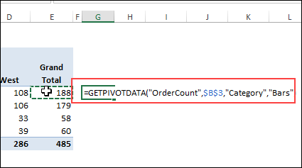
If you start the formula in cell G5, and then click on E5, Excel puts a long GetPivotData formula into the cell.
=GETPIVOTDATA(“OrderCount”,$B$3, “Category”, “Bars”)
And, if you didn’t notice that, and finished the division formula, here’s what Excel puts in the cell for you. Instead of normal cell references, there are two GetPivotData functions.
=GETPIVOTDATA(“OrderCount”,$B$3,”Category”,”Bars”) / GETPIVOTDATA(“OrderCount”,$B$3)
Copy the Formula Down
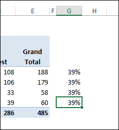
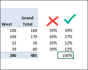
If you leave that GetPivotData formula as it is, and copy it down to the end of the pivot table, the result will be the same in every row. I’m sure that’s not what you wanted!
GetPivotData Function
The GetPivotData function is one of my favourite functions, but it’s annoying to have it automatically appear when you don’t need it.
As a temporary fix for the problem, you could simply type the cell references in your formula, instead of clicking on the pivot table values.
That will give you the correct results in each row, when you copy the formula down.
Turn GetPivotData Off
Instead of using a temporary fix, you can turn GetPivotData off, if you don’t need it. Here’s how to turn it off, so you get normal cell references:
- Select a cell in any pivot table
- On the Excel Ribbon, click the Analyze tab
- At the far left, click the Options arrow (or click the Pivot Table arrow, then click Options)
- Then, click the Generate GetPivotData command, to turn the feature on or off.

Global Setting
The Generate GetPivotData option is a Global setting in Excel. After you turn it off, Excel won’t automatically insert a GetPivotData function in any of your workbook.
If you ever need the feature again, just follow the same steps as above, and click the Generate GetPivotData command, to turn that option back on again.
________________________
Stop the Excel GetPivotData Formula
_________________________


