Excel Pivot Tables – Page 33 – by contextures.com

Change All Pivot Table Value Fields to SUM

Sometimes when you add fields to the Values area of a pivot table, they appear as Count of Field instead of Sum of Field. In the screen shot below, the Quantity field shows the COUNT, and the TotalPrice field shows the SUM.

pivot table Summary Macro_01

COUNT Summary Function

The COUNT summary function is the default if a field in the pivot table’s source data contains blank cells, or cells with text. For example, in a column of invoice dates, someone might mistype a month name, so it isn’t recognized as a valid date. Or, in a column of sales quantities, you might have typed “N/A”, instead of a number, or maybe you left a blank cell to fill in later.

In these cases, where the source column contains blank cells or text, the summary function defaults to Count; otherwise, it defaults to Sum.

Change the Summary Function

You can manually change the summary function from Count to Sum, after the Values fields have been added. Or, to make things easier, you can run a macro to change the summary function.

This sample macro changes all the Values fields in the first pivot table on the active sheet to use the Sum function (xlSum). The code refers to the pivot table by index number (1), instead of using a specific name (“PivotTable1”), and that makes the macro more flexible.

You can copy this code to a regular code module in your workbook, and run it when you want to change the summary functions for all the Value fields.

Sub SumAllValueFields()
  Dim pt As PivotTable
  Dim pf As PivotField
  Dim ws As Worksheet

  Set ws = ActiveSheet
  Set pt = ws.PivotTables(1)
  Application.ScreenUpdating = False

    pt.ManualUpdate = True
    For Each pf In pt.DataFields
      pf.Function = xlSum
    Next pf
    pt.ManualUpdate = False

  Application.ScreenUpdating = True
  Set pf = Nothing
  Set pt = Nothing
  Set ws = Nothing
End Sub

Download the Sample File

You can download the sample file with the Change Summary Function to Sum sample code, from my Contextures website.

The zipped file is in xlsm format, and contains macros. You can run the macro in the sample file, or copy the Excel VBA code to a regular code module in another workbook, and run it there.

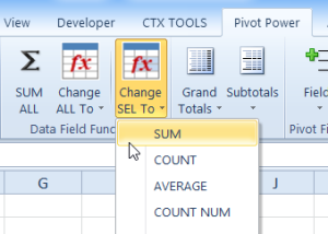
Pivot Power Add-in

If you’ve bought a copy of my Pivot Power Premium add-in, this feature is included. Just click the commands in the Data Fields group, and you can quickly change all fields to SUM, or any other summary function. Or, select specific value fields, and just change those to a different summary function.

sumselectedvalues

______________

Remove a Pivot Table Style in Excel 2007

When you create a pivot table in Excel 2007, a default PivotTable style is automatically applied to a pivot table. For example, in the screen shot below, the pivot table uses the Pivot Style Light 16.

Pivot Style Light 16

Remove the Pivot Table Style

In some workbooks, you might prefer to have a pivot table with no fill color or header formatting. In the PivotTable Styles gallery, you can apply a special style to remove the existing style.

Follow these steps to clear the PivotTable style:

Select a cell in the pivot table.
On the Ribbon, click the Design tab.
In the PivotTable Styles gallery, click the first style, None, at the top left of the Light styles.

Pivot Style None

Pivot Table Style Removed

After you click the None option, the existing style is removed, and a thin border remains around the pivot table sections. The worksheet gridlines, if displayed, are not visible within the pivot table.

Also, when no PivotTable style is applied, the preview function does not work if you point to a different style in the PivotTable Styles gallery.

Clear the Pivot Table Style

Another way to remove the PivotTable style is to click Clear, at the bottom left of the PivotTable Styles gallery.

Pivot Style Clear

______________

For more information on Pivot Tables, please see the Pivot Table Tutorials on the Contextures Website.

______________

Keep Formatting in Excel 2007 Pivot Table

Even though a pivot table is automatically formatted when you create it, you can add your own formatting later. For example, in the pivot table shown below, I’ve added colour to the subtotal rows, and made column B narrow.

PivotFormat01

However, some of that pivot table formatting might be lost if you refresh the pivot table or change its layout. Even if you select a different item in the report filter, the formatting could be lost.

Here’s what the same pivot table looks like, after I select an order date from the report filter.

Preserve the Formatting

Most pivot table formatting can be preserved if you change the Format options in the PivotTable Options dialog box.

Right-click a cell in the pivot table, and click PivotTable Options.
On the Layout & Format tab, in the Format options, remove the check mark from Autofit Column Widths On Update. This will prevent column widths from changing, if you have manually adjusted them.
Add a check mark to Preserve Cell Formatting on Update
Click OK.

PivotFormat03

Apply Formatting

After changing these Pivot Table options, the formatting should stick. When you apply formatting to the Pivot Table, do the following:

Ensure that Enable Selection is turned on.
Unless you want to format a single cell, use the pivot table selection technique to select the elements you want to format (point to the top or left edge of the element, and then click when the black arrow appears).

______________

P.S. For more information on Pivot Tables, please see the Pivot Table Tutorials on the Contextures Website.

_________________

Allow Drag-and-Drop in Excel 2007 Pivot Table

In Excel 2003, you could drag fields from the PivotTable Field List onto the pivot table layout on the worksheet.

In Excel 2007, you can only move the fields to the areas in the PivotTable Field List. In the screen shot below, if you try to drag the Promo field onto the pivot table, the cursor shows an X. The drag-and-drop feature doesn’t work.

PivotDrag01

Change the Pivot Table Settings

If you’d like to drag the pivot fields onto the worksheet layout, you can change a setting in the pivot table options.

Right-click a cell in the pivot table, and click PivotTable Options.
On the Display tab, add a check mark to Classic PivotTable Layout.
Click OK, to close the PivotTable Options dialog box.

Drag the Pivot Table Fields

After you change the setting, the pivot table on the worksheet shows a blue border around each region.

PivotDrag03

You can now drag the pivot fields from the PivotTable Field List onto the worksheet, or drag the fields to a different part of the pivot table.

Point to a field label in the pivot table layout
When the pointer changes to a four-headed arrow, drag the field label to a different area

PivotDrag04

You can use the same technique to drag fields into the pivot table layout from the PivotTable Field List, or drag field labels out of the pivot table layout.

Pivot Table in Tablular Form

When you change the setting to Classic PivotTable layout, the pivot table’s report layout automatically changes to Tabular form.

You can use Tabular form, or Outline form, with the Classic PivotTable layout. If you change to Compact form, the blue borders are still visible when the pivot table is active. However, you won’t be able to drag-and-drop the fields.

Video: Classic Layout

In this video, you’ll see the manual steps required to format a pivot table in Classic Style, so you can drag and drop the fields, right on the worksheet. There are several steps in the process:

change subtotal setting
change report layout of the pivot table
change pivot table style
change the pivot table display options
change setting to clear old items in Pivot Table
format each value field as number format
sort each row field alphabetically.

Save Time with a Macro: Near the end of the video, you’ll see how much quicker it is to run the recorded macro, to format the pivot able in seconds, instead of minutes. To get that macro, go to the Classic Layout Pivot Table Format Macro page, on my Contextures site.

___________________

Change Field Names in Pivot Table Source Data

Occasionally, you might need to change a column heading in the pivot table’s source data. For example, you could change a column heading from Qty to Quantity, to make it easier to understand.

Pivot Table Field Name 01

However, when you refresh the pivot table after making the changes, the renamed field will disappear from the pivot table layout. In our example, the Qty field is removed from the layout. It isn’t automatically replaced by the Quantity field, even though it’s in the same column heading cell in the source data.

Pivot Table Field Name 02

If you change the column headings, you’ll have to add the revised field to the pivot table layout again. If you had number formatting in the old pivot field, you’ll have to reapply the number formatting you had previously applied.

Change Captions Instead

If possible, instead of changing the column headings in the source data, create custom names for the fields in the pivot table instead.

For example, to create a custom name for the Qty field:

In the pivot table, click on the cell that contains the pivot field name, Qty.
Type the custom name, Quantity.
Press the Enter key, to complete the renaming.

Pivot Table Field Name 03

_____________________

For more information on Pivot Tables, please see the Pivot Table Tutorials on the Contextures Website.

_________________

PowerPivot For Excel 2010

Microsoft PowerPivot for Excel 2010 is a data analysis add-in for Excel 2010, and is part of the Office 2010 Beta. You can test PowerPivot in the hands-on Virtual Lab, or in the Office 2010 Beta, if you’ve downloaded that.

That’s where I tested PowerPivot last weekend, and described the experience in my Contextures blog article, Drill Into Data With PowerPivot.

There are step-by-step instructions in the module, and you can experiment a bit on your own too. For example, I tried a few of the Slicer formatting features.

You can connect each slicer to one or more of the pivot tables, and filter all the connected pivot tables at the same time.

_______________

See also: My PowerPivot for Excel 2010 Virtual Lab Review
For more information on PowerPivot, see the PowerPivot Team blog.
For a new pivot table formatting tip, see John Walkenbach’s Spreadsheet Blog: Unlinking A Pivot Table

___________________

Starting Each Pivot Item on a New Page

Normally, a long pivot table prints to the bottom of a page, then continues on the next page. The page break occurs naturally, not at a specific position in the pivot table.

You can control the page breaks, by changing the pivot table settings.

The Sample Layout

In this example, the pivot table has two fields in the Row Labels area – Store and Product Category.

pivotitempage01

We’d like to print this pivot table, with each store’s data starting on a new page. That way, we’d be able to print the entire
report, and send each store its own section.

Change the Field Setting

We’ll change a setting in the Store field, so each pivot item starts on a new page in the printed report.

Right-click one of the Store labels in the pivot table, and then click Field Settings.
In the Field Settings dialog box, on the Layout & Print tab, add a check mark to Insert Page Break After Each Item.
Click OK, to close the dialog box.

PivotItemPage02

Things to Consider

The Insert Page Break After Each Item setting doesn’t force all items for a field fit on one page. It only creates a page break so the next item will start on a new page. If a field has many items, it might print on two or more pages.

Also, with this setting, your printed report could use an excessive amount of paper. You might prefer to manually adjust the page breaks in Page Break Preview.

To Go To Page Break Preview

On the Ribbon’s View tab, in the Workbook Views group, click Page Break Preview.
Dashed lines indicate an automatic page break and solid lines are manual page breaks.
To move a page break, point to it, and drag up or down on the page.

To return to Normal view

On the Ribbon’s View tab, in the Workbook Views group, click Page Break Preview.

_____________

Pivot Table Defaults to Sum or Count

When you add a numeric field to the Values area of a pivot table, it usually appears as a Sum. For example, in the pivot table shown below, the Units field became Sum of Units.

ValueSum

Occasionally, when you add a numeric field to the Values area, it shows the Count, instead of the Sum. In the same pivot table, when the TotalSales field is added, it shows a Count.

ValueCount

Pivot Table Default Function

If you add a number field to the Values area, the default summary function is Sum. However, if the source data has blank cells, or nonnumeric data, such as text or errors, in that field, the Count function is the default summary function.

You can’t change the default settings for the data fields, but you can manually change the summary function after you add the fields to the Values area.

To manually change the summary function:

Right-click a cell in the field you want to change, and click Summarize Data By.
Click the summary function that you want to use.

SummarizeDataBy

Pivot Table Add-in

There’s a feature that changes all the data fields to SUM, or any other summary function, in my pivot table add-in. It add a new tab to the Ribbon, with time-saving commands that you can use.

After you install the add-in, select any cell in the pivot table.
Then, on the Ribbon’s Pivot Power tab, click SUM ALL.
Or, click Change ALL to, then click the Summary function that you want to use.

______________

For more information on Pivot Tables, please see the Pivot Table Tutorials on the Contextures Website.

_________________

New Pivot Items Out of Order

If you add new products to your pivot table source data, and refresh the pivot table, the new products will appear in the drop down lists. Sometimes though, the new items appear at the end of the list, instead of in alphabetical order. This problem can occur if you have manually rearranged the items in the Row Labels area.

For example, binders were just added to this pivot table’s source data. When the pivot table was refreshed, Binders appeared at the bottom of the Product list, instead of the top.

ListManualSort

Because it’s not in alphabetical order, it’s difficult to find the new product in the list. You’d like the product list sorted alphabetically.

Sort the List

If a field is set for Manual sort, new items will appear at the end of the drop-down list. Follow these steps to sort the field in ascending order:

Right-click a cell in the Product field. For example, right-click the Envelopes cell.
Click Sort, and then click Sort A to Z.

SortAZ

When you sort the Product field, its sort setting changes from Manual to Sort Ascending or Sort Descending. This also sorts the drop-down list, and makes it easier for users to find the items they need.

______________

For more information on Pivot Tables, please see the Pivot Table Tutorials on the Contextures Website. _________________

Re-create Pivot Table Source Data Table

If you accidentally delete the Excel 2003 worksheet that has the source data for your pivot table, you may be able to use the pivot table’s Drill to Details feature to re-create it.

Extract the Pivot Table Data

To re-create the source data in Excel 2003, follow these steps to use the Drill to Details feature:

Make sure that none of the items in the pivot table fields are hidden. For page fields, (All) should be selected. For row and column fields, (Show All) should be checked. Note: You don’t need to include all the fields in the pivot table before using the Drill to Details feature.
Show the grand totals for rows and columns. If they aren’t visible, right-click a cell in the pivot table, and click Table Options. Check the options Grand totals for rows and Grand totals for columns, then click OK.
Double-click the grand total cell at the bottom right of the pivot table. This should create a new sheet with the related records from the original source data.

Fix the Extracted Data

If the original source data contained formulas, you will have to re-create them, because the Drill to Details feature exports the data only.

The columns in the extracted data will be in the same order as they were in the original source data.

The extracted data will be formatted with Table AutoFormat List 3. You can apply a different AutoFormat, or apply your own formatting.

Note: If you had made changes to the source data and not updated the pivot table, those changes won’t be in the extracted data.

Connect to the Extracted Data

If you rename the sheet that was created during the Drill to Details process, and use the same name as the worksheet that originally held the source data, the pivot table might automatically connect to the new source data table.

If not, you can connect to the re-created source data:

Right-click a cell in the pivot table, and choose PivotTable Wizard.
Click the Back button, and select the new source data table range.
Click Finish.