Clear All Fields From a Pivot Table

Occasionally, you might want to tear down a pivot table, and start from scratch. You don’t have to delete the pivot table though – you can clear all the fields, and then start adding the ones you want.

Clear Pivot in Excel 2010

If you’re using Excel 2010 or 2007, it’s easy to clear the pivot table, using a Ribbon command.

  • Select a cell in the pivot table that you want to clear.
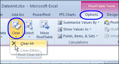
  • On the Ribbon, under PivotTable Tools, click the Options tab.
  • In the Actions group, click Clear, then click Clear All
RibbonClearAll

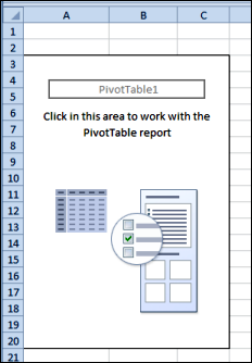
All the pivot fields are removed, and you’re left with an empty pivot table layout.
pivotempty

Undo the Clear

There’s no confirmation message when you click Clear All, so you can’t change your mind after you click that command.

However, you could click the Undo button, before performing any other actions, and all the pivot fields will be put back.

Clear the Pivot Table in Excel 2003

There’s no Clear All command in Excel 2003 and earlier versions, but you can manually remove the fields from the pivot table layout, either on the worksheet, or in the Pivot Table Wizard.

Clear the Pivot Table With Programming

The following code will clear all the fields from a pivot table, and make the field list visible, so you can start to rebuild it. Copy this code to a regular module in your workbook.

Note: You can’t undo the Clear All if you use this code. You could save the workbook before running the code, and then close without saving again, if you change your mind.

Sub ActiveCellClearPivot()
'clears pivot table for active cell
On Error Resume Next

Dim pt As PivotTable
Dim pf As PivotField

Set pt = ActiveCell.PivotTable
If Not pt Is Nothing Then

  pt.ManualUpdate = True
  
  'test version of Excel
  If CDbl(Application.VERSION) >= 12 Then
      'for Excel 2007 and later
      pt.ClearTable
  Else
    For Each pf In pt.VisibleFields
          pf.Orientation = xlHidden
    Next pf
  End If
  
  pt.ManualUpdate = False

  ActiveWorkbook.ShowPivotTableFieldList = True
End If

End Sub

_____________

Change Pivot Table Report Filters With VBA

With Report Filters at the top of your pivot table, you can select specific items from a field, and narrow the scope of your report.

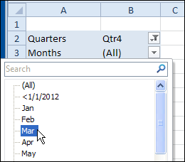
In the pivot table shown below, the order date field has been grouped, and Quarters and Months are in the Report Filter area.

reportfilterchangevba

Change Report Filters Automatically

I’ve previously posted sample code for changing one (or all) pivot table’s report filters, based on changes in another pivot table. In one of my Contextures Blog posts, Ian asked if we could change one report filter in a pivot table, based on another report filter in the same pivot table.

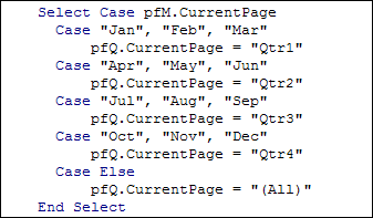
That sounded like an interesting challenge, so I’ve created code that changes the Quarters filter, when a month is selected. For example, if you select May, it will change to Qtr2. If your fiscal year is different, you could change the quarters in the code.

reportfilterchangevba02

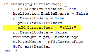
If you select a different Quarter, the Months filter will automatically change to "(All)". Then, if you want a specific month within that quarter, you could select it.

reportfilterchangevba03

Download the Sample File

To download the sample file, please visit the Pivot Tables VBA – Report Filters page on the Contextures website. The file is in Excel 2007/2010 format, zipped, and contains macros. Enable macros when you open the file, if you want to test the code.

In the file, to see the code, right-click on the pivot table sheet tab, and click View Code.

__________________

Filter All Pivot Tables for Specific Fields Only

On my Contextures website, there are a few sample files that let you filter one pivot table, and automatically change all the other pivot tables. You can find them on the Sample Files page, in the Pivot Table section.

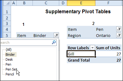
For example, in the worksheet shown below, if you select Pen Set as the Item in pivot table 1, the same item will be selected in pivot table 2.

pivotfiltermultilist02

This works with Excel VBA Event code, that runs automatically when either pivot table is updated.

Limit the Filter Fields

This code works well, if you want to change all of the fields in all of the workbook’s pivot tables. However, you might have a different worksheet for each Region’s pivot table. If someone changes a Region on one sheet, you don’t want it to automatically change all the other sheets.

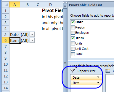
In the latest version of the Change Multiple Pivot Tables Automatically workbook, I’ve added a sheet where you can select the specific fields that you want to include. In the screen shot shown below, the Master List pivot table only has Date and Item in its Report Filter area.

pivotfiltermultilist01

Change the Filter

With the revised code, if you filter one of the pivot tables for Region, only that pivot table will be affected, because Region is not in the master list. If you filter for Item or Date, all the pivot tables in the workbook will be updated with the selected item.

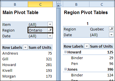
In the screen shot below, Region is being changed in the worksheet at the left. The change will not affect the worksheet on the right. However, if the Date is filtered in either pivot table, it will automatically update the other pivot tables in the workbook.

pivotfiltermultilist03

Download the Sample File

To see the code and test the macro, please visit the Excel Sample Files page, and go to the Pivot Tables section. Look for PT0028 – Change Specific Page Fields with Multiple Selection Settings, and download the zipped file.

The file is in Excel 2007/2010 format, and it contains macros. Be sure to enable macros if you want to test the code.

__________________

Check for Shared Pivot Cache

Last year, I posted Excel VBA code for removing a calculated field from a pivot table.

The code works well if there is only one pivot table based on that pivot cache. However, a couple of comments mentioned that there were problems if multiple pivot tables shared the pivot cache.

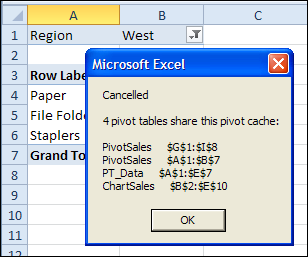
Here is a revised version of the code, that checks for other pivot tables using the same pivot cache. If others are found, the macro is cancelled, and a message appears, listing the pivot tables.

pivotcancelmessage 

Remove Calculated Fields for Non-Shared Pivot Cache

If other pivot tables in the workbook share the same cache, the macro is cancelled. A message lists those pivot tables.

Sub RemoveCalculatedFieldsNotShared()
Dim ws As Worksheet
Dim ptA As PivotTable
Dim pt As PivotTable
Dim pf As PivotField
Dim pfNew As PivotField
Dim strSource As String
Dim strFormula As String
Dim iPC As Long
Dim lCache As Long
Dim strPC As String


Set ptA = ActiveSheet.PivotTables(1)
iPC = ptA.PivotCache.Index

For Each ws In ActiveWorkbook.Worksheets
    For Each pt In ws.PivotTables
        If pt.PivotCache.Index = iPC Then
            lCache = lCache + 1
            strPC = strPC & ws.Name & "     " _
                & pt.TableRange2.Address _
                & vbCrLf
        End If
    Next pt
Next ws

If lCache > 1 Then
    MsgBox "Cancelled" _
        & vbCrLf & vbCrLf _
        & lCache & " pivot tables share this pivot cache: " _
        & vbCrLf & vbCrLf _
        & strPC
    GoTo exitHandler
Else
    For Each pf In ptA.CalculatedFields
        strSource = pf.SourceName
        strFormula = pf.Formula
        pf.Delete
        Set pfNew = ptA.CalculatedFields.Add(strSource, strFormula)
    Next pf
End If

exitHandler:
    Exit Sub

End Sub

_______________

Quickly Change Pivot Table Data Functions

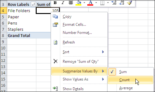
It’s easy to change the summary function for one data field in a pivot table. For example, if a field shows the Sum of Units, you can right-click on that field, and change it to Count of Units.

pivottablesummaryfunctions02

However, if you have several data fields in a pivot table, it can take quite a bit of time to change each pivot table summary function manually.

Create a Worksheet List of Functions

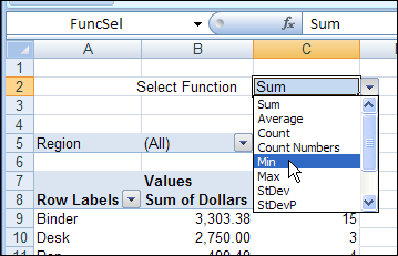
To make it easy for yourself, or other people who use the pivot table, to change the functions, you can add a drop down list of functions in a worksheet cell.

PivotFunctionChange02

The list is created with Excel data validation, and Excel VBA code runs when a different function is selected in that cell. The code changes the summary function for all the data fields in the pivot table.

Read the Details

For details on how the code works, you can read the Select Pivot Table Function From Worksheet Drop Down article on the Contextures blog.

Download the Sample File

To test the Summary Function code, you can download the sample file from the Contextures blog link above. The file is in xlsm format, and zipped. Enable macros when you open the file.

________________

Clean Up Pivot Table Show Details Sheets

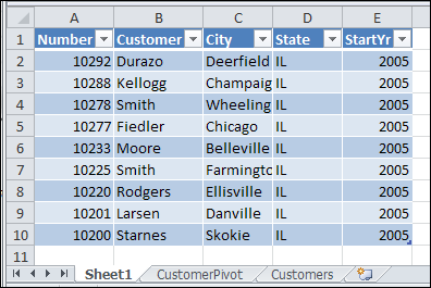
When you double-click on the value cell in a pivot table, a new sheet is automatically inserted in the workbook. The new sheet contains a table, listing all the source data records that are summarized in the number that you double-clicked.

showdetails03

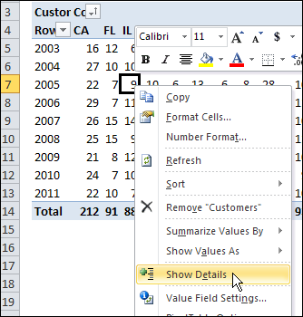
Double-clicking the cell is a shortcut to the pivot table Show Details command. You can also right-click on a value cell, and click Show Details.

showdetails02

Show Details, also called DrillDown, is a great feature for digging into the details, but you can end up with lots of extra sheets in your workbook.

However, you don’t usually want to save the sheets, so you manually delete them before you close the file.

Automatically Name the Sheets

With event code on the pivot table’s worksheet, and in the workbook module, you can add a prefix, such as “XShow”, when the Show Detail sheets are created.

showdetails06

That prefix should make the sheets easier to find and delete, before you close the workbook.

Automatically Delete the Sheets

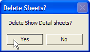
To make the cleanup task even more efficient, you can use programming to show a message when you’re closing the workbook, if there are Show Details sheets in the file.

showdetails04

If you click Yes, all the sheets with the “XShow_” prefix are deleted, and the workbook stays organized. Then, save the tidied up version of the workbook, when prompted.

See the Drilldown Sheet Code

For detailed instructions on adding the drilldown sheet naming and deleting code, visit the Excel Pivot Table Drilldown page on the Contextures website.

Download the Sample Drilldown File

To see how the event code names the sheets, and deletes them when closing, you can download the sample file from my Contextures website, at the link shown above.

________________

Make Pivot Table Macros Run Faster

Pivot table macros can run painfully slowly, even if you have turned off screen updating and disabled events.

To make the code run faster, you can try adding a line that turns off automatic updating in the pivot table. For example:

     Set pt = Worksheets("PivotSales").PivotTables(1)

pt.ManualUpdate = True

At the end of the code, you can reverse the setting, to turn automatic updating on:

     pt.ManualUpdate = False

Watch the Pivot Table Video Tutorial

In this short video, you can see that the pivot table macro runs much faster when the ManualUpdate setting is changed.

Note: In Excel 2007, the macro won’t run if the Defer Layout Update setting is checked. This problem is fixed in Excel 2010.

____________

Pivot Table Calculated Field Removed with Excel VBA

If you’re working with pivot table calculated fields in Excel VBA programming, or trying to use the Orientation property for data fields, you might encounter some problems. Here’s how I managed to work around an error that occurs for a pivot table calculated field removed with Excel VBA.

Continue reading “Pivot Table Calculated Field Removed with Excel VBA”

Pivot Table From Data in Multiple Workbooks

To create a pivot table from data on different worksheets, you can use a Multiple Consolidation Ranges pivot table, but the result is a pivot table with limited features and functionality.

Previously, Excel MVP Kirill Lapin shared his macro for creating a standard pivot table from data on different worksheets.

Now Kirill has expanded that technique, and written a macro to build a pivot table from data in multiple Excel files.

Pivot Table Macro

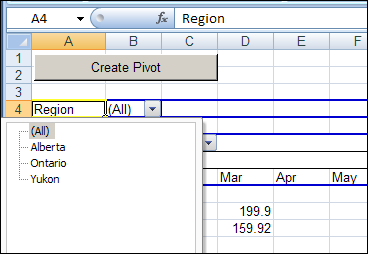
In Kirill’s example, the main file is named Report.xls. It contains the pivot table code, and a button that runs the macro. After you start the macro, it prompts you to select one or more data files, all stored in the same folder.

All of the data files must have the same structure, and the macro pulls the data stored on Sheet1 in each file.

Standard Pivot Table

The macro creates a standard pivot table based on a Union query, and not built from Multiple Consolidation Ranges, it’s a fully functioning pivot table, and you can pivot, group and filter the data, as usual. You can also refresh the pivot table, to show the latest data in the source files, as long as those files stay in their original location.

pivotwkbk04

The Union Query

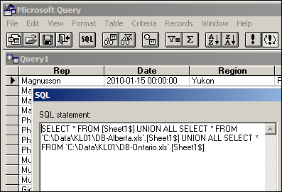
Kirill’s macro creates a Union query to combine the data from all the selected files. If you open Microsoft Query, you can see the SQL string for the Union query, and all the data from the selected workbooks.

pivotwkbk05

Download the Sample File

You can download the Pivot Workbooks example to see the sample code and create the pivot table. The zipped folder that contains the Report.xls file, and the five sample data files. Unzip the folder, and keep all the files in the same folder. When you open the Report.xls file, enable macros to run the code.

______________

Identify an Excel Pivot Table Pivot Cache

If you have an Excel workbook that contains several pivot tables and multiple Excel Tables, you might want to identify which pivot cache each pivot table uses.

To figure out which pivot cache a pivot table uses, you can use a macro to check the pivot table’s CacheIndex property and show the index number in a message box.

Add the Pivot Cache Code

The following Excel macro will show the pivot cache index number for the selected pivot table. Copy the code and paste it into a regular code module in an Excel workbook.

Sub ViewCacheIndex()

On Error GoTo err_Handler

MsgBox "PivotCache: " & _
    ActiveCell.PivotTable.CacheIndex
Exit Sub

err_Handler:

MsgBox "Active cell is not in a pivot table"
End Sub

Run the Pivot Cache Code

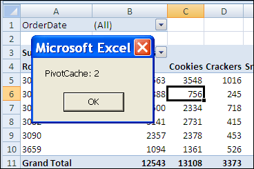
Select a cell in a pivot table, and then run the macro. A message box displays the CacheIndex property for the active cell’s pivot table.

pivotcache01

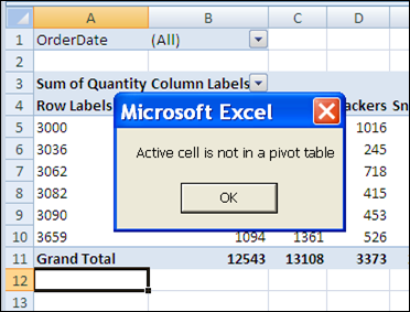
If the active cell is not in a pivot table, an error message is displayed.

pivotcache02

How the Macro Works

When a a pivot cache is created, it is added to the workbook’s PivotCaches collection and given an index number. That index number is displayed in the macro’s message box. If a pivot table is based on the same source data as an existing pivot table, it uses the same pivot cache.

__________