Usually you can only show numbers in a pivot table values area, even if you add a text field there. In the screen shot below, the Max of Region ID is in the Values area.
Instead of the numbers 1, 2 or 3, we’d like to see the name of the region – East, Central or West.
When you show subtotals for a pivot table date field, the dates might not be formatted like the rest of the dates. We’ll take a look at why this happens, and how you can fix it.
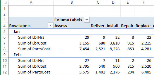
For example, in the screen shot below,
the date (in row 4) is formatted as d-mmm-yy
the subtotal date (in row 8) is formatted as mmm/yy
When you create a pivot table from your source data, it only shows the items that have data. For example, if you put Customers and Products in the Row area, it only lists the items that each customer has bought.
Most of the time, you probably use a pivot table on your computer, but occasionally you might need to print one, to share with other people in your company.
Onscreen, pivot tables can get quite wide, and you can scroll back and forth, to see everything. In the pivot table shown below, there are 3 Values fields, and they are repeated for each of the items in the Column field.
When you add fields to the row labels area in a pivot table, the field’s items are automatically sorted. See how you can manually move those labels, to put them in a different order. There’s a video and written steps below.
A pivot table shows a summary of the source data, and in the screen shot below you can see all the products that were sold, and the quantities for each colour.
When you filter the pivot table, some of that data might disappear. For example, in the pivot table shown below, the Customer field has been filtered to show XYZ Inc. orders.
They didn’t order all the colours for each product, so the pivot table is smaller. It’s only showing the products and colours that XYZ Inc. ordered.
Instead of having the pivot table change size, so it shows only the applicable items, you can change a field setting, to keep it consistent.
Show All Items in Excel 2010
To make all the items appear, even if the pivot table is filtered, you can change a Layout setting in the pivot table. This setting applies to a single field, so you’ll have to make the following change to each field in which you want to see all the items.
To show all items for a pivot field in Excel 2010 or 2007:
Right-click an item in the pivot table field, and click Field Settings
In the Field Settings dialog box, click the Layout & Print tab.
Check the ‘Show items with no data’ check box.
Click OK
After the setting is changed, all the colours are listed for each product, even if they weren’t sold for the selected customer.
To see the instructions for changing the setting in Excel 2003, please go to my Contextures website: Pivot Table Field Settings
Watch the Video
Watch this video to see the steps for changing the layout setting in Excel 2010 or 2007.
In Excel 2003, and earlier versions, when you added multiple data fields to a pivot table, they were automatically arranged vertically. The data headings showed up in the Row area, stacked one on top of the other.
Here is the same pivot table, with horizontal data headings.
Vertical Data in Excel 2010 Pivot Table
Pivot tables changed quite a bit in Excel 2007, and the default layout for multiple data fields is now horizontal. Using the same data, this is the default layout in Excel 2010.
If you want to change the data to a vertical layout, you can drag the Values button in the Pivot Table Field List, from the Column Labels area to the Row Labels area.
Usually, the Values button would be positioned below the other fields in the Row Labels area.
After you move the Values label, the data fields will be rearranged, and they will show vertically, with headings in the Row Labels area.
Watch the Excel 2010 Data Layout Video
To see the steps for rearranging the data in Excel 2010, please watch this short video tutorial.
When you have a long list of fields in an Excel 2003 pivot table, it can take a long time to drag them into the pivot table layout, using the PivotTable Wizard.
For a quicker way to add the fields, don’t go into the Layout screen in Step 3 — just click the Finish button.
Add Fields from the PivotTable Field List
When the PivotTable Wizard closes, you’ll see a blank pivot table on the worksheet.
Note: If the PivotTable Field List isn’t visible, click the Show Field List button on the PivotTable Toolbar.
To add the pivot fields:
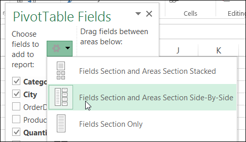
Then, in the Field List, select one of the layout areas from the drop down list.
In the Field List, double-click on each field that you want to add to the selected layout area.
Repeat Steps 1 and 2, for all the layout areas, leaving the Data Area to fill in last.
In the PivotTable Field List, the fields usually appear in the same order that they appear in the source data. If the pivot table source data has lots of fields, it might be hard to find a specific field in the list.
To make it easier to find the fields in the long list, you would like the field list in alphabetical order.
Sort the List
You can change a pivot table option, to make the PivotTable Field List show the fields in alphabetical order.
Right-click a cell in the pivot table, and in the pop-up menu, click PivotTable Options.
In the PivotTable Options dialog box, click the Display tab.
At the bottom of the Display tab, in the Field List section, select Sort A to Z, and then click OK
Later, if you want to return the field list to its original order, select Sort in Data Source Order, instead of Sort A to Z.