In a pivot table, there’s no built-in way to group the pivot table data by both weeks and months at the same time. If you want to show sales data by week, you can group the date field in seven-day intervals.
The 7 day grouping works well, but if you try to add grouping by months, the Number of Days option is disabled. If you select Month in the Grouping dialog box, the days will lose their 7 day grouping.
Calculate the Month
Since you can’t group by both week and month, you can use a workaround instead. You could create a column in the source data, and then calculate one of the grouping levels there. Then, you could add that field to the pivot table.
For example, you can add a column that calculates the month name for each sales order date, by using the TEXT function:
=TEXT(A2,"mmm")
Add the Month field to the pivot table, above the weeks.
Calculate the Week Number
Another option is to add a column to the source data, with a formula to calculate the week number:
=WEEKNUM(A2).
With the OrderDate field in the Row Labels area, group the dates by months. In the Row Labels area, add the WeekNum field below the OrderDate field, to summarize the data by month and week number.
Note: If a week begins in one month and ends in another, it will appear under both months.
You can create a calculated field in a pivot table, to perform calculations based on the Sum of a pivot table field. For example, the formula below would calculate a bonus based on the total number of units sold for each product.
When you add a field to the Values area of an Excel Pivot Table, it automatically shows the Sum or Count for all the items in that field. Here we can see the total labor cost for each Service Type.
If you add more than one field to the Row Labels or Column Labels area of the Pivot Table, a subtotal is automatically created for each field except the last one (the Inner Field). The subtotal, by default, uses the same summary function as the Value field.
In our example, the District field has been added to the Row Labels area. Service Type is now an Outer Field, and has a subtotal for each service. District is the Inner Field, and does not have subtotals.
Change the Subtotal Summary Function
Instead of using the default summary function for subtotals, you can select a different function. To change the setting:
Right-click a label for the field in which you want to change the subtotal. In this example, right-click cell B3, which has the Install label.
In the pop-up menu, click Field Settings
In the Field Settings dialog box, click the Subtotals & Filters tab
Under Subtotals, click Custom
In the list of Summary Functions, click one or more function names
Click OK to close the dialog box.
Subtotals on Inner Fields
For the Inner Field in the Row Labels or Column Labels area, the default subtotals are not displayed. So, in the pivot table shown above, there’s no subtotal for the District field.
However, if you create Custom Subtotals for an Inner Field, those subtotals appear at the end of the Pivot Table. In this example, Custom subtotals for Count and Max were created for the District field. You can see the District subtotals at the bottom of the Pivot Table, just above the Grand Total.
More Info on Pivot Table Subtotals
You can read more about pivot table subtotals, and the steps for changing them, on the Contextures website: Excel Pivot Table Subtotals.
Watch the Pivot Table Subtotals Video
To see the steps for changing the pivot table subtotals, and creating multiple subtotals, you can watch this short video.
If you format a column of dates in your pivot table source data, to show as year and month (yyyy-mm), they won’t automatically summarize by year and month in the pivot table.
Format the Source Data
For example, in the source data shown below, there are several orders for January 2010, and three different dates are visible.
If you format those records as yyyy-mm, it looks like all the dates are the same.
Summarize Formatted Dates
However, when you add the OrderDate field to the Row Labels area of a pivot table, several items appear as 2010-01, instead of only one item.
The first instance of 2010-01 shows 3 orders, so that would be the Jan 2, 2010 orders. Below it is an item with a single order, and that’s a summary of the Jan 3, 2010 orders.
Even though the dates are formatted to look the same in the source data, the underlying dates are still recognized by the pivot table. Those underlying dates are used for the pivot table summary. If you click a date in the Row Labels, you see the underlying date in the formula bar. Because the dates are different, each date is listed individually.
Group the Dates
Instead of formatting, you can group the dates in the pivot table to combine the data by month and year.
Right-click an OrderDate row label, and then in the context menu, click Group.
In the Grouping dialog box, in the By list, select Months and Years, and then click OK.
The orders will be grouped by year and month, showing a total of 38 for January 2010.
Calculate the Year and Month
Grouping can cause some problems in a pivot table, such as preventing you from using calculated items. If you don’t want to using grouping, you could add a new column to the source data, and enter a formula that converts the dates to text. Then, all the dates that have the same year and month will calculate to the same text string.
In our example, the order dates are in column A.
Add a blank column to the source data table, with the heading YrMth.
In the cell below the heading, type the formula =TEXT(A2,”yyyy-mm”)
Copy the formula down to the last row of data in your table. (Note: If your data is in an Excel Table, the
formula should fill down automatically.
Refresh the pivot table, so you can see the new YrMth field in the PivotTable Field List.
Add the YrMth field to the pivot table Row Labels area.
Remove the old OrderDate field from the pivot table layout.
The orders are grouped by year and month, showing a total of 38 for January 2010.
However, the grouping options are based on the calendar year, and there are no options for grouping pivot table dates by fiscal year. If you want to group the dates by your company’s fiscal year, which starts in July, there’s no built-in way to do that.
Pivot Table dates grouped by year and quarter
Fiscal Year Workaround
Because there’s no built-in option to group pivot table dates by fiscal year, you’ll have to use a workaround solution. In the pivot table source data, you can add a column with a formula that calculates the fiscal year, and then add that field to the pivot table.
For example, if your fiscal year starts in July, use the following formula to calculate the fiscal year, where the date is in cell A2:
=YEAR(A2)+(MONTH(A2)>=7)
The formula calculates the year of the date in cell A2. Then, it calculates the month of the date in cell A2, and checks to see if the month number is 7 or higher. If the month is less than 7, then zero will be added to the year, otherwise 1 will be added.
In the screenshot below, you can see the fiscal year formula for dates in June and July.
The year for all the dates is 2010.
For the June dates, the month is 6, which is less than 7. So, zero is added to the year, and the fiscal year is 2010.
For the July dates, the month is 7, so 1 is added to the year, and the fiscal year is 2011.
Fiscal Year formula
Fiscal Quarter Workaround
If you also want to group the pivot table dates by the fiscal quarter, you can add another column to the pivot table source data. Use this formula to calculate the fiscal quarter, if the fiscal year starts in July.
=CHOOSE(MONTH(A2),3,3,3,4,4,4,1,1,1,2,2,2)
The Choose formula calculates the month of the date in cell A2. Based on the month number, the formula selects the appropriate fiscal quarter number from the numbers that follow. For example, if the month is June, the month number is 6. In the Choose formula, the sixth number is 4, so June is in fiscal quarter 4.
In the screenshot below, you can see the fiscal quarter formula for dates in June and July.
For the June dates, the month is 6, and the sixth month in the Choose formula is 4, so June is in fiscal quarter 4.
For the July dates, the month is 7, and the seventh month in the Choose formula is 1, so July is in fiscal quarter 1.
fiscal quarter formula for dates in June and July
Add the Fiscal Dates to the Pivot Table
If you had grouped year and quarter dates in the pivot table, ungroup them and remove them.
Refresh the pivot table, and add the fiscal year and fiscal quarter fields to the Row Labels area.
fiscal year and fiscal quarter fields in pivot table
Videos: Pivot Table Grouping
Learn more about pivot table grouping, and get a workbook with sample file that you can use for testing. Go to the How to Group Pivot Table Data page on my Contextures website.
First, this video shows how to group Text items in a pivot table.
Next, this short video shows the basics of pivot table grouping
______________
When you add a date field to your Pivot Table, Excel automatically groups the dates into a hierarchy, such as years and months. See how to stop pivot table date grouping in the latest versions of Excel, and a couple of workarounds for Excel 2016. You can also read about why this feature was added, and watch a date grouping video.
Prevent Date Grouping
It’s easy to prevent automatic date grouping for pivot tables in Excel 2019/365, by changing a setting. See the simple steps below.
If you’re using Excel 2019 or Excel for Office 365, there’s good news. You don’t have to use workarounds or make changes to the registry. Now, you can simply change one of the Excel options, to stop pivot table date grouping.
NOTE: This is an application-level setting, not a setting for individual workbooks.
To turn this setting off:
At the top of Excel, click the File tab
Click Options, then click the Data category
In the “Data options” section, add a check mark to “Disable automatic grouping of Date/Time columns in PivotTables”
Click OK to close Excel Options
Excel 2016 Workaround
In Excel 2016, there isn’t an easy way turn off pivot table date grouping. However, to prevent dates from automatically grouping in Excel 2016, you can use this 2-step workaround:
Add the date field to the pivot table Report Filter area first. Dates are not automatically grouped there
Then, in the PivotTable Fields list, drag the date field into the Rows or Columns area. Dates will remain ungrouped.
Excel 2016 Registry
The only way to turn off pivot table date grouping in Excel 2016, if you’re brave enough, is by making a change to the Windows Registry.
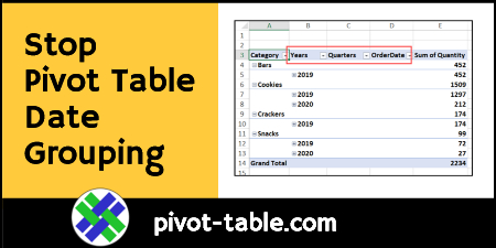
Pivot Tables dates weren’t grouped in earlier versions of Excel, but that behaviour changed in Excel 2016. Since that version, dates in Pivot tables have been automatically grouped too.
Here’s a pivot table in which I added the Category and OrderDate fields to the Rows area. Because of the date grouping, extra columns were automatically created, to show the Years and Quarters, as well as the Order Date.
Implementing grouping for Data Model PivotTables allows for grouping to be used in conjunction with the power of the xVelocity engine and is a key feature for making Data Model PivotTables a replacement for native ones in the future. When used in a data model PivotTable, Time grouping adds relevant Date/Time columns such as Date (Year), Date (Quarter) and Date (Month) to the grouped table in the model; these columns could then be reused with other user endpoints of the data model, such as PowerView and Power BI
The date grouping feature can help in normal pivot tables too. For example, with a large dataset, Excel shows an error message if I try to put the date field into the Columns area.
“You cannot place a field that has more than 16384 items in the column area. If you want to use this field in the report, click OK, and then move the field to either the row area or page area.”
However, Excel allows me to put the Date field into the Rows area, and it automatically groups the dates into Years and Quarters. That saves me the step of having to group the dates manually.
The new fields – Years and Quarters are also automatically added to the PivotTable Fields list.
With these grouped fields, I can move Years into the Columns area, and Excel won’t show an error message about the item limit.
Undo Pivot Table Date Grouping
So, the date grouping feature can be a real time saver, if you usually group the dates manually. But, if you don’t like the grouping feature, there are steps you can take to undo it or stop it, depending on which version of Excel you’re using.
For all versions (Excel 2016 and later), you can manually ungroup the dates, with one of these methods:
Keyboard Shortcut
Add the Date field to the pivot table
Immediately press Ctrl + Z, to undo the automatic date grouping
The grouped fields are removed, and the original Date field remains in the pivot table
Ungroup Command
Add the Date field to the pivot table
At any time, right-click on any of the date field items or headings
In the right-click menu, click Ungroup
The grouped fields are removed, and the original Date field remains in the pivot table
Video: Pivot Table Date Grouping
Watch this video to see how to group the date field in 4-week periods, and set the starting date. There are written instructions on my Contextures website – Group Pivot Table Dates
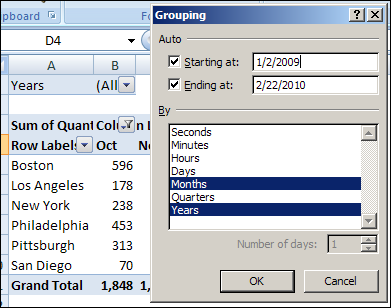
For example, in a pivot table with sales order data, you can group the Order Date field by years and months, to quickly compare the sales totals each month, for a selected year.
group dates by years and months
In this pivot table example, we have sales data for six stores. Three of the stores are new, and opened in the past 12 months. The other 3 stores are older. You’re doing a presentation to the Board of Directors, and you’d like to compare the sales in the new stores to sales in the older stores.
The new stores are in:
Los Angeles
Philadelphia
San Diego
The older stores are in:
Boston
New York
Pittsburgh
To group the Order Date field, you clicked on one of the dates in the pivot table, then clicked Group Field on the Ribbon’s Option tab.
Group Field on the Ribbon’s Option tab
However, when you click a label in the City field, the Group Field command isn’t available, so you aren’t sure how to create the Old and New groups for the City field.
Group the Selected Items
The Group Field command is only available for date and number fields in the Row Labels or Column Labels area of the pivot table.
Because the City names are entered as text, you can use a different method to group them.
Manually select the cities you want in the first group. To select nonadjacent cities, hold the Ctrl key, and then click the city names.
In this example, we’ll select the cities with the new stores, Los Angeles, Philadelphia and San Diego.
select text items to group them
With the city names selected, on the Ribbon’s Options tab, click Group Selection
click the Group Selection command
Name the Group
This creates a new item in the City field, named Group1, with the selected cities listed under that heading. For each of the remaining cities, a heading is created, with its city name.
Group1 created in pivot table
To change the name of the new group, click on the Group1 heading cell, and then type a name for the group, such as New Stores.
change name of new group
Group the Remaining Items
Next, you can group the remaining stores and name that group.
Select the remaining stores, and click the Group Selection command to group them.
Select the remaining stores
Name the second group as Old Stores.
Alternative Method of Grouping
Instead of grouping the stores in the pivot table, you could add a StoreType field to the source data, and then enter Old or New for each record.
Next, add the new StoreType field as the first field in the Row Labels area. The city names will appear under the correct StoreType heading.
Videos: Pivot Table Grouping
Learn more about pivot table grouping, and get a workbook with sample file that you can use for testing. Go to the How to Group Pivot Table Data page on my Contextures website.
First, this video shows how to group Text items in a pivot table.
Next, this short video shows the basics of pivot table grouping
______________
For more information on Pivot Tables, please see the Pivot Table Tutorials on the Contextures Website.
When you add multiple fields to the Row Labels area in a pivot table, subtotals automatically appear for the outer fields. In the pivot table shown below, Region and City fields are in the Row Labels area. Two fields are in the Values area: Sum of Quantity shows the total quantity for each city, and Sum of TotalPrice shows the total sales amount.
Region Subtotal is Shown
A subtotal row is at the bottom of each region. It shows the total quantity and total sales for each region. You can add another row of subtotals for each region, to show the average quantity and sales.
Add More Subtotals
You can change the field settings for the Region field and it will show more subtotal rows:
Right-click one of the Region row labels, and click Field Settings.
In the Field Settings dialog box, click the Subtotals & Filters tab.
In the Subtotals section, click Custom. Note: When you select Custom, the Automatic subtotal is removed.
In the list of functions, click Sum and Average – the functions you want to use as subtotals.
Click OK, to close the Field Settings dialog box
Note: When you select multiple Custom subtotals, the subtotals are displayed at the bottom of the group, even if you set the option to show subtotals at the top of the group.
When you add multiple fields to the row or column area, the outer fields automatically get subtotals. For example, in this pivot table, Region and Employee are the outer fields, and a Total row was added for each item.
Sometimes these subtotals are useful, but in other pivot tables you might want to stop them from appearing.
Manually Turn Off the Subtotals
Unfortunately, here’s no setting you can change to stop the subtotals from automatically appearing for outer row and column fields. However, you can manually turn them off after they appear:
1. Double-click the field button.
2. For Subtotals, select None, then click OK.
Programmatically Turn Off the Subtotals
If you frequently turn off the subtotals, you might find it easier to use a macro to do the work for you. You can create your own code, or purchase my Pivot Power Premium add-in
It has commands to show or hide the Row, Column, or all Subtotals in a pivot table.
In your source data, you might record the amount of time that employees have spent working on projects. For example, Jim worked on Project A for 8 hours Monday, 8 hours Tuesday, 6 hours Wednesday and 3 hours Thursday, for a total of 25 hours.
In the pivot table, you want the total time per project, and Project A should show a total of 25 hours.
However, your pivot table shows 1:00 as the total, instead of 25:00.
This happens because the results are shown as time rather than total time. The first 24 hours are counted as one day, and the remaining hour is 1:00 AM of the second day. The 1:00 in the Project A Total represents the 1:00 AM time.
To see the total time, format the cells that contain total times with the custom number format [h]:mm, and they’ll total correctly.
To apply the custom format
In the pivot table, right-click on the Sum of Hours field button
Click on Field Settings
Click the Number button
In the Category list, click on Custom
In the Type box, enter: [h]:mm
Click OK, twice, to close the dialog boxes.
The pivot table will now show the total time for hours worked on each project.
___________________________
For more information on pivot tables, see the PivotTable Topics on my Contextures web site.