A quick way to show how amounts accumulate over time is to build a pivot table, and show the values as a running total.
However, if you group the dates by year and month, the running total stops at the end of each year, and starts again at the start of the next year. There is no setting you can adjust to change this behavior.
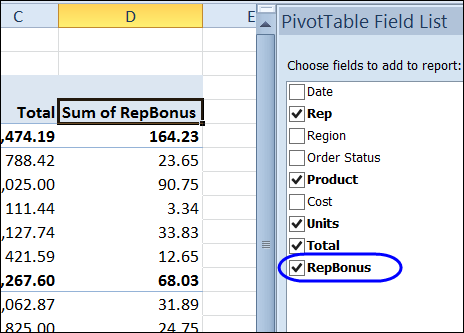
Besides using the fields from a pivot table’s source data, you can create calculated fields. These fields are formulas that can refer to other fields in the pivot table, to perform calculations on the summarized amounts.
In this example, the RepBonus calculated field is added to the pivot table, to show the bonus amounts paid on product sales.
It’s easy to create a running total in a pivot table, and it’s usually used to show how quantities accumulate over time.
In this example, there are three Value fields in the pivot table, showing the number of units sold on each date.
In column B, the Sum of Units is shown, with no calculation. This is the number of units sold on each date listed.
In column C, the Sum of Units is shown, as a Running Total for Date. This is the total units sold, up to and including each date.
In column D, the Sum of Units is shown, as % Running Total for Date (new in Excel 2010). This is the total units sold, up to and including each date, divided by the grand total of units sold.
Running Total for Date
When you select either Running Total In or % Running Total In, you have to select a Base Field. The running totals will be accumulated at each change in that Base Field.
We want a running total down the list of dates, so Date is the Base field in this example.
By November 1st, a running total of 399 units have been sold, and the % Running Total is 18.8% of the 2121 overall total units sold.
End of Year Problems
The running total works for a continuous list of dates, but doesn’t flow down the whole list if you group the dates by years and months. In the pivot table shown below, the date has been grouped by Years and Months.
Now the running totals stop at December 2012, and start again in January 2013.
It can be a little difficult to understand the running totals in this layout, so be sure to label the pivot table headings, or add a title to explain it.
You might have used one of the Custom Calculations in a pivot table, such as % of Column or Running Total. There’s another Custom Calculation – Index — that isn’t used very often, but provides an interesting look at the pivot table values.
In the screen shot below you can see the original data in the pivot table, and the same date using the Index custom calculation. Even though Central Auto is the highest value in the table at the left, East Property has the highest Index value.
Using the Index custom calculation gives you a picture of each value’s importance in its row and column context.
If all values in the pivot table were equal, each value would have an index of 1.
If an index is less than 1, it’s of less importance in its row and column
If an index is greater than 1, it’s of greater importance in its row and column.
The Index Formula
Even if two cells have the same value, they may have a different index. The Index formula is:
So, in this example, in the West region, the values for Auto and Property are almost equal, but the index for the Auto is 1.02 and Property is 0.98.
Because the grand total is higher for the Property column, the Grand Column Total in the Index formula is larger. The West Property amount is divided by this larger number, and its resulting index is smaller.
In a pivot table, you can create calculated items, in addition to the pivot items from the source data. They can create problems in your pivot table layout, such as showing cities under every region, instead of just the region in which they’re located.
In this tutorial, I’ll create a calculated item in the Category field, and then fix the problem that it creates in the City field.
Pivot Table Setup
In the pivot table shown below, the Category field is in the Column headings, and it is filtered to show only two of the four categories – Crackers and Snacks.
The Region and City fields are in the Row headings, and there are 3 cities in the East and 2 cities in the West.
Create a Calculated Item
I want to add a new Category – Sweets – to show the total for the two hidden categories – Cookies and Bars.
To create the Calculated Item:
Select one of the Category heading cells, such as cell D4.
On the Ribbon, under PivotTable Tools, click the Options tab
In the Calculations group, click Fields, Items & Sets, and click Calculated Item
Type a name for the calculated item – Sweets
In the Formula box, enter the formula: =Bars + Cookies
Click OK, to Add the new item, and to close the Calculated Item window.
Calculated Item Problems
After you click OK, the Sweets category is added to the pivot table, in the Column Headings, as expected. However, each city is now listed under each region, with zero amounts in some rows.
What Went Wrong
When you add a calculated item, all the items are listed for fields that intersect the calculated item. The calculated item creates every possible combination of items in the intersecting fields, even if there is no data for that combination in the source data.
Unfortunately, you can’t change this behaviour – there’s no setting to turn it off. If possible, avoid calculated items, which can slow down a large pivot table, and create calculations in your source data instead.
Hide the Zero Rows
To hide the cities that are in the wrong region, you can use a pivot value filter to hide the rows with a zero total.
Note: This will also hide any other rows with zero grand total, so use this technique with caution.
Right-click a cell that contains a City row label, and in the context menu, click Filter, and then click Value Filters.
In the Value Filter window, from the first drop-down list, select Qty, which is the Values field you want to check.
In the second drop-down list, select does not equal
In the third box, type 0 (zero), and then click OK
The rows where the grand total is zero are hidden, and the wayward city names disappear from each region.
To extract data from an Excel Pivot Table, you can use the GetPivotData function. Unless you change the default settings, a GetPivotData formula is automatically created if you type an equal sign, and then click on a pivot table data cell, to link to it.
In the screen shot below, I typed an equal sign in cell A3, and then clicked on cell D7, which contains the total sales for:
Region: West
Product: Paper
Date: Dec 1st
The GetPivotData formula that was automatically created is:
Instead of leaving the text values in the formula, you can replace those values with cell references. This makes the formula flexible, and it will show a different result, based on the values in the linked cell.
For example, I’ve entered a region name in cell A1, a product name in cell B1, and a date in cell C1.
Then, in the formula, I replaced “West” with a link to cell A1, and replaced “Paper” with a link to cell B1.
The formula result will now change automatically if I type East in cell A1, and type Pens in cell B1.
Create a Date Cell Reference
It’s a little trickier to create a cell reference for a date. Instead of just clicking on the date cell, you’ll use cell links within the DATE function.
The arguments for the DATE function are: year, month, day. In the original formula, the selected date is shown as: DATE(2012,12,1)
You can use the YEAR, MONTH and DAY functions to pull those values from the date in cell C1. The completed formula with flexible cell references is:
In addition to the regular items in a pivot table, you can also create calculated items, in one or more of the pivot fields.
In this pivot table, we’re summarizing data about insurance policies, with the number of new, cancelled, and existing policies in five regions.
Instead of showing all the data, we need to show the cancellation rate in the Northeast and the Southwest. To do this, we’ll add three calculated items, and those formulas will overlap in some of the cells. And that can lead to some problems!
Add Calculated Item for Cancellation Rate
First, we’ll hide the “New” status, and the “Central” region, by removing the check marks for those items in the field drop down lists.
Next, we’ll create a calculated item in the Status field, for cancellation rate:
Click on one of the labels in the Status field, such as cell A6.
On the Excel Ribbon, under PivotTable Tools, click the Options tab
In the Calculations group, click Fields, Items & Sets, and click Calculated Item.
In the Insert Calculated Item dialog box:
Type a name for the calculated item – CancelRate
Enter the formula: = Cancel/( Cancel+ Existing)
Click OK, to add the item.
In the pivot table, the CancelRate row will appear as zeros, so format those values as percentage, with one decimal place.
If you click on one of the cells in the CancelRate row, you’ll see the CancelRate formula that is used in the cell.
Add Calculated Item for Regions
Next, we’ll create calculated items for the Northeast and the Southwest, to show totals for the regions in those areas.
To create a calculated item for the Northeast:
Click on one of the labels in the Region field, such as cell B4.
On the Excel Ribbon, under PivotTable Tools, click the Options tab
In the Calculations group, click Fields, Items & Sets, and click Calculated Item.
In the Insert Calculated Item dialog box:
Type a name for the calculated item – Northeast
Enter the formula: = North + East
Click Add, to add the item, and keep the dialog box open.
To create a calculated item for the Southwest :
Type a name for the next calculated item – Southwest
Enter the formula: = South + West
Click OK, to add the item, and close the dialog box.
In the pivot table, drag the Northeast label to the left, so it is beside the North region.
Incorrect Cancellation Rates
The Northeast and Southwest columns are showing totals for the Cancel and Existing values, and those numbers are correct.
However, the CancelRate item is also being summed, which is not what we want. For example, the Northeast CancelRate shows 11.7%, which is the total of 5.9% + 5.8%.
Instead, we want that rate calculated as it is in East: = Cancel/( Cancel+ Existing). The rate should be 5.8%.
If you click on the Northeast CancelRate cell, the Northeast formula is showing, instead of the CancelRate formula.
Change the Solve Order
To fix the problem, you can change the Solve Order for the calculated items:
Select a cell in the pivot table, and then on the Ribbon, under PivotTable Tools, click the Options tab
In the Calculations group, click Fields, Items & Sets, and click Solve Order.
The message at the bottom of the Calculated Item Solve Order dialog box explains that the last formula listed is the one that determines the cell’s value.
We’ll move CancelRate to the bottom, so its formula will be used in the CancelRate row.
Click on the CancelRate item, and click the Move Down button, twice, to move it to the bottom of the list.
Click Close
Note: When you change the Solve Order, it affects all calculated items in the pivot table.
The Correct Results
With the Solve Order changed, the percentages in the CancelRate row are now showing the correct values – 5.8% for the Northeast and 2.7% for the Southwest.
When you click on the Northeast CancelRate cell, the CancelRate formula is showing, so the solve order change has fixed the problem.
Download the Sample File
To download the Solve Order, please visit the Calculated Item page on my Contextures website.
Watch the Video
To see the steps for creating calculated items, and changing the solve order, please watch this short video.
With a pivot table, you can quickly summarize data, and show the Sum or Count for thousands of records. For example, in the pivot table shown below, the weekly regional sales are shown.
Besides showing a basic sum or count for the data, you can use custom calculations, to show things like a running total, or the differences between items in a pivot field.
Right-click on a value cell in a pivot table, then click Show Values As, to see a list of custom calculations that you can use.
Calculate the Difference
One that I use frequently is the Difference From custom calculation, that subtracts one pivot field value from another, and shows the result.
Note: If you want to show the difference between pivot fields, instead of pivot items, you can create a calculated field.
In the pivot table below, a second copy of the Units field has been added to the pivot table, and it shows the difference from the sum of one week’s sales to the next.
Change the Summary Function
You can use different summary functions with a custom calculation — not just a Sum. In the example shown below, the Units field is added to the Values area twice.
Both copies of the Units field are set to show the Count summary function.
The second copy of the Units field is changed to a custom calculation for Difference From.
Custom Calculation Tips
If you’re using custom calculations, here are a few tips to make them more effective.
To make the data easier to understand, you can change the heading from “Sum of Units” to “Units Change”.
You can add another copy of the Units field to the pivot table, and show both the total sales and difference in weekly sales
Experiment with the pivot table layout, to find the arrangement that will be easiest to read and understand.
Remember that a custom calculation can only calculate on items within the same pivot field. If you want to show the difference between pivot fields, instead of pivot items, you can create a calculated field.
Watch the Difference From Video
To see the steps for creating a Difference From custom calculation, please watch this short video tutorial.
Download the Sample File
To test the Difference From custom calculation, you can download the sample file from my Contextures website: Custom Calculations
When you add fields to a pivot table, you can show or hide that field’s pivot items. In addition to the existing items, you can create calculated items for a pivot field.
In the screen shot below, the Order Status field has 4 items – Backorder, Canceled, Pending and Shipped.
To combine the amounts for Backorder, Pending and Shipped, you could create a calculated item – Sold.
Then, hide the other items, and just show Canceled and Sold in the pivot table, under the Order Status field.
Watch the Video
To see the steps for creating a calculated item, and displaying it in the pivot table, please watch this short video tutorial. You’ll also hear the disadvantages to using calculated items.