Category: Calculations

After you create a calculated field in an Excel pivot table, you might want to remove it from the pivot table layout. You can temporarily remove a calculated field, or you can permanently remove it.

In this example, the pivot table has a calculated field named Bonus. It appears in the Values area as Sum of Bonus. You could hide the Bonus calculated field, or delete it from the pivot table.

Temporarily Remove a Calculated Field

To temporarily remove a calculated field from a pivot table, follow these steps:

1. In the pivot table, right-click a cell in the calculated field. In this example, we’ll right-click the Bonus field.
2. In the popup menu, click the Remove command that shows the name of the calculated field.

The calculated field is removed from the pivot table layout, but remains in the PivotTable Field List.

Later, you can add a check mark to the calculated field in the PivotTable Field List, to return it to the pivot table layout.

Permanently Remove a Calculated Field

To permanently remove a calculated field, follow these steps:

1. Select any cell in the pivot table.
2. On the Ribbon, under the PivotTable Tools tab,  click the Options tab.
3. In the Tools group, click Formulas, and then click Calculated Field.
4. From the Name drop down list, select the name of the calculated field you want to delete.
   • 
5. Click Delete, and then click OK to close the dialog box.

______________

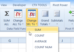
For more information on Pivot Tables, please see the Pivot Table Tutorials on the Contextures Website.

______________

Sometimes when you add fields to the Values area of a pivot table, they appear as Count of Field instead of Sum of Field. In the screen shot below, the Quantity field shows the COUNT, and the TotalPrice field shows the SUM.

COUNT Summary Function

The COUNT summary function is the default if a field in the pivot table’s source data contains blank cells, or cells with text. For example, in a column of invoice dates, someone might mistype a month name, so it isn’t recognized as a valid date. Or, in a column of sales quantities, you might have typed “N/A”, instead of a number, or maybe you left a blank cell to fill in later.

In these cases, where the source column contains blank cells or text, the summary function defaults to Count; otherwise, it defaults to Sum.

Change the Summary Function

You can manually change the summary function from Count to Sum, after the Values fields have been added. Or, to make things easier, you can run a macro to change the summary function.

This sample macro changes all the Values fields in the first pivot table on the active sheet to use the Sum function (xlSum). The code refers to the pivot table by index number (1), instead of using a specific name (“PivotTable1”), and that makes the macro more flexible.

You can copy this code to a regular code module in your workbook, and run it when you want to change the summary functions for all the Value fields.

Sub SumAllValueFields()
  Dim pt As PivotTable
  Dim pf As PivotField
  Dim ws As Worksheet

  Set ws = ActiveSheet
  Set pt = ws.PivotTables(1)
  Application.ScreenUpdating = False

    pt.ManualUpdate = True
    For Each pf In pt.DataFields
      pf.Function = xlSum
    Next pf
    pt.ManualUpdate = False

  Application.ScreenUpdating = True
  Set pf = Nothing
  Set pt = Nothing
  Set ws = Nothing
End Sub

Download the Sample File

You can download the sample file with the Change Summary Function to Sum sample code, from my Contextures website.

The zipped file is in xlsm format, and contains macros. You can run the macro in the sample file, or copy the Excel VBA code to a regular code module in another workbook, and run it there.

Pivot Power Add-in

If you’ve bought a copy of my Pivot Power Premium add-in, this feature is included. Just click the commands in the Data Fields group, and you can quickly change all fields to SUM, or any other summary function. Or, select specific value fields, and just change those to a different summary function.

______________

When you add a numeric field to the Values area of a pivot table, it usually appears as a Sum. For example, in the pivot table shown below, the Units field became Sum of Units.

Occasionally, when you add a numeric field to the Values area, it shows the Count, instead of the Sum. In the same pivot table, when the TotalSales field is added, it shows a Count.

Pivot Table Default Function

If you add a number field to the Values area, the default summary function is Sum. However, if the source data has blank cells, or nonnumeric data, such as text or errors, in that field, the Count function is the default summary function.

You can’t change the default settings for the data fields, but you can manually change the summary function after you add the fields to the Values area.

To manually change the summary function:

1. Right-click a cell in the field you want to change, and click Summarize Data By.
2. Click the summary function that you want to use.

Pivot Table Add-in

There’s a feature that changes all the data fields to SUM, or any other summary function, in my pivot table add-in. It add a new tab to the Ribbon, with time-saving commands that you can use.

1. After you install the add-in, select any cell in the pivot table.
2. Then, on the Ribbon’s Pivot Power tab, click SUM ALL.
3. Or, click Change ALL to, then click the Summary function that you want to use.

______________

For more information on Pivot Tables, please see the Pivot Table Tutorials on the Contextures Website.

_________________

After you create a calculated item in a pivot table, you might need to change its formula.

For example, in this pivot table there’s a calculated item named Sold, in the Order Status field. The Sold item sums the orders with a status of Shipped, Pending, or Backorder.

Change the Calculated Item Formula

You can change the formula, so it doesn’t include the Backorder items. To do that, follow these steps to go back into the Insert Calculated Item dialog box and modify the calculated item.

1. In the pivot table, one of the Order Status items. For example, select cell A6, which is the Canceled item.
2. On the Ribbon, click the Options tab, under the PivotTable Tools tab.
3. in the Tools group, click Formulas, and then click Calculated Item.
4. In the dialog box, click the drop down arrow for the Name box.
5. Select Sold, which is the name of the calculated item you want to change.
6. In the Formula box, change the formula, to remove the +Backorder.
7. The revised formula is =Shipped+Pending.
8. Click Modify, to save the change, and then click OK to close the dialog box.

_________________

If you’ve used calculated items and calculated fields in your pivot table, you can automatically create a list of all the formulas.

List the Formulas in Excel 2007

1. Select any cell in the pivot table.
2. On the Ribbon, under the PivotTable Tools tab, click the Options tab.
3. In the Tools group, click Formulas
4. Click  List Formulas.

A new sheet is inserted in the workbook, with a list of the calculated fields and a list of the calculated items.

List the Formulas in Excel 2003

1. Select any cell in the pivot table.
2. On the Pivot toolbar, click PivotTable.
3. Click Formulas, then click  List Formulas.

A new sheet is inserted in the workbook, with a list of the calculated fields and calculated items (see the Excel 2007 example above).

___________________________

For more information on pivot tables, see the Pivot Tables on my Contextures web site.

___________________________

If there are blank cells in one of the fields in your source data, you might want to show a count of the blank cells in the pivot table.

In this example there’s a Region field in the source data, and some of the records have no region name entered. In the pivot table, you’d like to see a count of how many records are missing a region name.

NOTE: For an updated version of this article, go to Count Blank Entries in Pivot Table

Incorrect Count

To find the count, you might add the Region field to the pivot table’s row area, and put another copy of the Region field in the data area, as Count of Region.This seems logical, but there’s no count showing for the blank regions.

Video: Count Blank Entries in Pivot Table

[Update] This 3-minute video shows the steps for correctly counting blank items from the source data for a pivot table.

Get the sample Excel file, and written steps, on the Count Blank Cells in Pivot Table page on my Contextures site.

Get Correct Count

A pivot table can’t count the blank cells when you add a field to the data area and use the Count or CountNum summary function. That’s why no count appears beside the (blank) region in the screen shot above.

Instead, put a different field in the data area, and use it for the count.

For example, if the Units field will always contain data, add Count of Units to the data area, as shown below.

The count of blank Regions is now calculated, and you can see that three records are missing a region name.