Debra – Page 37 – Excel Pivot Tables

Deleting the Entire Pivot Table

To remove a pivot table from an Excel workbook, you can delete the worksheet that the pivot table is one.

Occasionally, you might want to remove a pivot table, but you can’t just delete the worksheet because it contains other data. To remove a pivot table, and leave the other items on the sheet untouched, you can clear the cells.

Clear the pivot table cells

1. Select a cell in the pivot table

2. On the menu bar, click Edit|Clear|All.

3. On the PivotTable toolbar, click PivotTable|Select|Entire Table

This will remove the pivot table, and all its formatting, from the worksheet.

Note: After deleting the pivot table, you might temporarily see drop down arrows where the pivot fields were located, but these should disappear when you activate another cell.

___________________________

For more information on pivot tables, see the Pivot Table Topics on my Contextures web site.

___________________________

Changing Blank Row Labels

In your Excel pivot table, you might have a few row labels or column labels that contain the text “(blank)”.

This happens when data is missing from the source data. For example, in the source data, you might have a few sales orders that don’t have a Store number entered.

Labels Show (Blank)

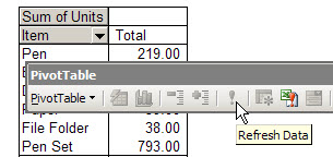
In the pivot table shown below, there is one store number cell, in column A, that shows (blank).

Instead of that text, you want blank cells in the Row Labels area and Column Labels area to contain the text “N/A.”

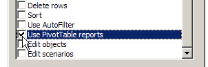
In the PivotTable Options dialog box, on the Layout & Format tab, you entered N/A as the text to display in empty cells, and then you clicked the OK button.

However, the empty cells still appear as (blank) in the Row and Column Labels areas.

Does NOT Change Labels

In the PivotTable Options dialog box, the setting for empty cells:

affects cells in the Values area
does NOT affect the Row or Column Labels areas.

In the screen shot above, you can see that missing data in the Values area has been replace by N/A, but the row labels and column labels haven’t changed.

Manually Change Blank Labels

You can manually change the (blank) labels in the Row or Column Labels areas by typing over them in the pivot table.

You can type any text to replace the (Blank) entry, but you CANNOT clear the cell and leave it empty.

How to Change Label Text

Here are the steps for manually changing a pivot table row label text or labels in the column areas. I used “N/A” in this example, but you could use a different text string, or a space character.

To change a blank label cell to “N/A”, follow these editing steps:

First, select one of the Row or Column Labels that contains the text (blank).
- Even if there are multiple cells with a “(blank)” label, you only need to select one of them.
- You DO NOT need to press Ctrl and select all of them
Next, on your keyboard, type N/A in the cell, and then press the Enter key.

Note: All other (Blank) items in that same pivot field will change to display the same text, N/A in this example.

___________________________

More Pivot Table Tips

For more information on pivot tables, see these pages on my Contextures site:

Manually Move Pivot Items

Clear Old Items in Pivot Table

Pivot Table Options

_________________

Refreshing When a File Opens

In Excel 2003, if your pivot table source data changes frequently, you might want to ensure that the pivot table is updated as soon as the file opens.

You can set a pivot table option to refresh the pivot table automatically:

Right-click a cell in the pivot table, and choose Table Options.
Under Data options, add a checkmark to Refresh on open.
Click OK to close the PivotTable Options dialog box.

Tip: To stop a long refresh, as the file opens press the Esc key.

___________________________

For more information on pivot tables, see the Pivot Table Topics on my Contextures web site.

Totaling Hours in a Pivot Table Time Field

In your source data, you might record the amount of time that employees have spent working on projects. For example, Jim worked on Project A for 8 hours Monday, 8 hours Tuesday, 6 hours Wednesday and 3 hours Thursday, for a total of 25 hours.

In the pivot table, you want the total time per project, and Project A should show a total of 25 hours.

However, your pivot table shows 1:00 as the total, instead of 25:00.

This happens because the results are shown as time rather than total time. The first 24 hours are counted as one day, and the remaining hour is 1:00 AM of the second day. The 1:00 in the Project A Total represents the 1:00 AM time.

To see the total time, format the cells that contain total times with the custom number format [h]:mm, and they’ll total correctly.

To apply the custom format

In the pivot table, right-click on the Sum of Hours field button
Click on Field Settings
Click the Number button
In the Category list, click on Custom
In the Type box, enter: [h]:mm
Click OK, twice, to close the dialog boxes.
The pivot table will now show the total time for hours worked on each project.

___________________________

For more information on pivot tables, see the PivotTable Topics on my Contextures web site.

Add Running Totals to an Excel Pivot Table

With a running total in a pivot table, you can see how amounts accumulate over a period of time, or through a range of products, as shown in the short video below.

In the video, the pivot table contains monthly sales figures for several products, and we’ll create a running total by month. In the pivot table, Date is in the row area, grouped by month. Product is in the column area, and Units sold, shown as Sum of Units, is in the data area.

This is what the pivot table looks like before we add the Running Totals custom calculation.

Follow these steps to add a Running Total:

Right-click on one of the data cells, and click on Field Settings.
Click the Options button.
From the dropdown list for Show data as, select Running Total In.
For the Base field, select Date, then click the OK button.

Note: If you select a base field that isn’t in the row or column area, all the results will show an #N/A error.

For more examples of Running Totals, please visit Pivot Tables — Running Totals

___________________________

For more information on pivot tables, see the Pivot Table Topics on my Contextures web site.

Remove Old Items in Excel 2007 Pivot Table

To prevent old items from being retained in an Excel 2007 pivot table, you can change an option setting, as shown in the short video below:

Right-click a cell in the pivot table
Click on PivotTable options
Click on the Data tab
In the Retain Items section, select None from the drop down list.
Click OK, then refresh the pivot table.

Details at www.contextures.com/xlPivot04.html

___________________________

For more information on pivot tables, see the Pivot Table Topics on my Contextures web site.

Use the Chart Wizard to Create a Pivot Chart

In Excel 2003, if you select a cell in the pivot table and click the Chart Wizard button on the Standard toolbar, a default pivot chart on a chart sheet is created. In some cases you might prefer to step through the Chart Wizard so you can set the options as you create the pivot chart.

Create a Pivot Chart with the Chart Wizard

Select an empty cell away from the pivot table and any other data on the worksheet.
On the Standard toolbar, click the Chart Wizard button.
In Step 1 of the Chart Wizard, select a Chart type and Chart sub-type, then click Next.
In Step 2 of the Chart Wizard, click in the Data range box, then select any cell in the pivot table. The entire pivot table will be automatically selected, and its address will appear in the Data range box.
Continue through the Chart Wizard steps, selecting the options you want, then click Finish to create the pivot chart.

Note: After selecting a pivot table as the data range, you can’t return to Step 2 of the Chart Wizard. To use a different data range, create a new chart.

___________________________

For more information on pivot tables, see the Pivot Table Topics on my Contextures web site.

Selecting Sections of an Excel Pivot Table

When working with a pivot table, you might want to select a specific section, such as the subtotals, or a set of labels. In this short video I use the Selection Arrow to select specific sections of an Excel Pivot Table.

I also show you how to turn on the Enable Selection feature, if you can’t see the Selection Arrow when working with pivot tables on your computer.

For more information on pivot tables, see the Pivot Table Topics on my Contextures web site.

Turn Off GetPivotData Formulas for PivotTables

In Excel 2002, and later versions, when you type an equal sign, then click on a data (number) cell in a pivot table, you may see a GETPIVOTDATA formula, instead of a cell reference.

GetPivotData formula

In this short video, learn how to turn this feature off.

For written instructions, please see Turn Off GetPivotData Formulas for Excel Pivot Tables.

___________________________

Refreshing a Pivot Table on a Protected Sheet

In Excel 2003, if you protect a worksheet, you’ll see a list of options, with specific items that can be allowed.

You can add a checkmark to “Use PivotTable reports”, so that people will be able to use the existing pivot tables on the worksheet.

protect worksheet settings

However, once the sheet is protected, you can’t create a new pivot table. Also, you won’t be able to refresh a pivot table on the worksheet, because that feature is disabled on a protected sheet. On the PivotTable toolbar, you can see that the Refresh button, and other features, are disabled.

pivot table toolbar with buttons disabled

Refresh the Pivot Table on a Protected Sheet

To refresh the pivot table on a protected worksheet,

temporarily unprotect the worksheet,
refresh the pivot table,
protect the sheet.

You can do this manually, or record a macro, then run that macro to refresh the pivot table.

More Protection Tips

There are more pivot table protection tips on my Contextures website.

___________________________