Filter All Pivot Tables for Specific Fields Only

On my Contextures website, there are a few sample files that let you filter one pivot table, and automatically change all the other pivot tables. You can find them on the Sample Files page, in the Pivot Table section.

For example, in the worksheet shown below, if you select Pen Set as the Item in pivot table 1, the same item will be selected in pivot table 2.

pivotfiltermultilist02

This works with Excel VBA Event code, that runs automatically when either pivot table is updated.

Limit the Filter Fields

This code works well, if you want to change all of the fields in all of the workbook’s pivot tables. However, you might have a different worksheet for each Region’s pivot table. If someone changes a Region on one sheet, you don’t want it to automatically change all the other sheets.

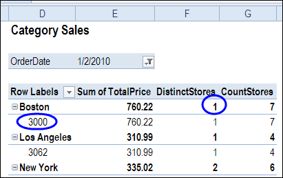
In the latest version of the Change Multiple Pivot Tables Automatically workbook, I’ve added a sheet where you can select the specific fields that you want to include. In the screen shot shown below, the Master List pivot table only has Date and Item in its Report Filter area.

pivotfiltermultilist01

Change the Filter

With the revised code, if you filter one of the pivot tables for Region, only that pivot table will be affected, because Region is not in the master list. If you filter for Item or Date, all the pivot tables in the workbook will be updated with the selected item.

In the screen shot below, Region is being changed in the worksheet at the left. The change will not affect the worksheet on the right. However, if the Date is filtered in either pivot table, it will automatically update the other pivot tables in the workbook.

pivotfiltermultilist03

Download the Sample File

To see the code and test the macro, please visit the Excel Sample Files page, and go to the Pivot Tables section. Look for PT0028 – Change Specific Page Fields with Multiple Selection Settings, and download the zipped file.

The file is in Excel 2007/2010 format, and it contains macros. Be sure to enable macros if you want to test the code.

__________________

Change Excel Pivot Table Subtotal Text

When you add two or more fields to the Row area in a pivot table, the outer fields will automatically display subtotals. By default, the subtotal row has a label that stars with the item name, followed by "Total"

In the pivot table shown below, the Category and Product fields are in the Row Labels area, and there is a subtotal for each item in the outer field – Category. You can see the Bars Total and Cookies Total labels.

pivotsubtotaltext01

Instead of leaving the default subtotal labels, you type a new label in any subtotal row. The text that you enter will apply to all the subtotals in that field.

Type a New Subtotal Label

When you type a new subtotal label, you can include the item name, or omit it. For example, if you select the Bars Total label in cell A9, and type "Subtotal", all of the items will change to that label. There is no item name in any subtotal label.

pivotsubtotaltext02

Include the Item Name

If you include the item name, such as Subtotal – Bars, when typing the new text, each subtotal will include its own item name.

pivotsubtotaltext03

When you type the item name, be sure to type it exactly as it appears in the pivot table. If you misspell the item name, such as "Bar" instead of "Bars", that word will be included in all the other subtotal labels.

pivotsubtotaltext04

Text Before and After Item Name

You can add text before and/or after the item name in the subtotal label. In the next example, the Bars subtotal label was changed to, "This is the Bars Subtotal". The other products show the same text before and after their item names.

pivotsubtotaltext07 

Get Creative with Subtotals

In addition to text, you can use other characters in the subtotal labels. In the example below, I typed a couple of space characters, then equal signs and a greater than symbol, to create an arrow.

pivotsubtotaltext05 

In the next example, I pressed the Alt key, and typed 16 on the numeric keypad, to create a right-pointing triangle. That certainly draws attention to the subtotals!

pivotsubtotaltext06 

NOTE: If you’re using a keyboard that doesn’t have a separate numeric keypad, you might have to press the Fn key, and the Alt key, then type 16 on the numbers that appear on the JKL keys.

So, you can get creative with those subtotal labels. Just remember that they can’t be changed individually – a change to one will be applied to all of them.

_____________________

Arrange Pivot Table Data Vertically

In Excel 2003, and earlier versions, when you added multiple data fields to a pivot table, they were automatically arranged vertically. The data headings showed up in the Row area, stacked one on top of the other.

piv04a

If you wanted the data headings arranged horizontally, you could drag the data button in the Column area.

Here is the same pivot table, with horizontal data headings.

piv05

Vertical Data in Excel 2010 Pivot Table

Pivot tables changed quite a bit in Excel 2007, and the default layout for multiple data fields is now horizontal. Using the same data, this is the default layout in Excel 2010.

pivotdatavertical01

If you want to change the data to a vertical layout, you can drag the Values button in the Pivot Table Field List, from the Column Labels area to the Row Labels area.

pivotdatavertical02

Usually, the Values button would be positioned below the other fields in the Row Labels area.

pivotdatavertical03

After you move the Values label, the data fields will be rearranged, and they will show vertically, with headings in the Row Labels area.

pivotdatavertical04

Watch the Excel 2010 Data Layout Video

To see the steps for rearranging the data in Excel 2010, please watch this short video tutorial.

_____________

Pivot Table Grand Totals at Top

When you create an Excel pivot table, the grand totals are automatically added at the bottom, and at the right. With the Grand Total command on the Excel Ribbon, you can show or hide the grand totals, but you can’t move them.

The good news is that there is a quick and easy workaround for this problem, which allows you to show the column grand total at the top.

There are written instructions on my Contextures website, on the Pivot Table Grand Totals page, where you can also download a sample file for this technique.

Watch the Grand Totals Video

To see the steps for the grand total workaround, please watch this short video.

__________________

Create Multiple Copies of Excel Pivot Table

In an Excel pivot table, you can put fields in the Report Filter area, like the City and YrMth fields in the pivot table shown below.

image

If you need to print a report for a specific city, you can select that city’s name from the drop down list.

image

Create a Pivot Table for Each City

If you want to print a copy of the pivot table for each city in the drop down list, it might take a while to do the task manually. Instead, you can use a built-in pivot table feature, to automatically create a separate pivot table for each city. Each pivot table will be on its own worksheet, and will have all the formatting that you applied to the original pivot table.

To create a pivot table for each item in a pivot table’s Report Filter:

  1. In the City filter, select "(All)", or select specific cities from the list. If a city is not selected, a pivot table copy will not be created for it.
  2. Select a cell in the pivot table, and on the Excel Ribbon, under the PivotTable Tools tab, click
    the Options tab.
  3. At the left end of the Ribbon, click the drop down arrow for Options.
  4. Click Show Report Filter Pages
    •  image
  5. In the Show Report Filter Pages dialog box, click on City, to select that field.
    • image
  6. Click OK, to create the pivot table pages.

A worksheet is created for each city, with the city’s name on the sheet tab. On each worksheet
is a copy of the original pivot table, with the city’s name selected in the Report Type filter.

image

Print the City Pivot Tables

After you create the City pivot table pages, you can select all the City worksheets, and print them.

Then, while the City sheets are still selected, delete them, so only the original pivot table is left in the workbook.

image

More Pivot Table Tips

Please visit the Contextures website for more Excel pivot table tips and tutorials.

________________________

Unique Count in Pivot Table With Excel PowerPivot

In Excel 2010, there is no built-in summary function that calculates a distinct count or unique count in a pivot table. In the pivot table shown below, we’d like to see the number of stores in Boston, where each product category was sold.

Continue reading “Unique Count in Pivot Table With Excel PowerPivot”

Sorting Pivot Table Report Fields

To focus on specific data in an Excel pivot table, you can add a field to the Report Filter area. Then, select one or more items from that pivot table field, to see the summarized data.

If you put a date field in the Report Filter area, there might be a long list of dates in the dropdown list. When you create the pivot table, the dates are usually in ascending order, with the oldest dates at the top of the list.

That’s not too convenient, if you want to focus on the latest data, instead of the oldest. How can you change the sort order, to put the newest dates at the top of the list?

Sort the Report Filter Field

Usually, it’s easy to sort a pivot table field. For example, if you right-click on a field in the Row area, the popup menu shows sorting and grouping options.

PivotFilterGroup01

However, when you right-click a Report Filter field, those sorting and grouping options aren’t listed in the popup menu.

PivotFilterGroup02

Move the Pivot Table Field

To solve the sorting problem, you can use a workaround – temporarily move the Report Filter field to the Row Labels area.

PivotFilterGroup03

Then, use the right-click popup menu to sort the date field in descending order.

PivotFilterGroup04

Drag the field back to the Report Filter area, after you sort it.

PivotFilterGroup05

Report Filter Dates in Descending Order

After you sort the field in descending order, you’ll see the latest dates at the top of the drop down list.

PivotFilterGroup06

It’s not the ideal solution, but it works! Maybe in the next version of Excel you’ll be able to sort the fields, without moving them from the Report Filter area.

Video: Sort Report Filter Field

Watch this very short video, to see how to show the items alphabetically, by temporarily moving the Report Filter field to the Rows area in the pivot table.

Download the Sample File

To download the sample file, please visit the Pivot Table Sorting page on my Contextures website.

_________

Repeat Pivot Table Labels in Excel 2010

When you create a pivot table in Excel 2010 or Excel 2007, the row labels are in a compact layout – all the headings are listed in column A.

PivotLabelRepeat01

You can change the Report Layout setting, to either Outline form or Tabular form, so each row field is in a separate column.

PivotLabelRepeat02

Here’s the same pivot table in Outline form. The Region field is in column A, with a separate row for each new heading.

PivotLabelRepeat04

Repeat the Row Labels

A new feature in Excel 2010 lets you repeat those row labels, so they appear on every row in the pivot table.

To turn on that feature for all the fields, select the Repeat All Item Labels on the Ribbon’s Design tab.

PivotLabelRepeat03

Here’s the pivot table in Outline form, with repeating row labels.

PivotLabelRepeat05

Repeating Labels for a Single Field

Instead of turning on repeating labels for the entire pivot table, you can apply the feature to a specific pivot table field.

In this example, the Region, City and Store fields are in the Row area, and we’ll turn on repeating labels for the Region field only.

  1. Right-click one of the Region labels, and click Field Settings
  2. In the Field Settings dialog box, click the Layout & Print tab
  3. Add a check mark to Repeat item labels, then click OK

PivotLabelRepeat06

Now, the Region labels are repeated, but the City labels are only listed once.

PivotLabelRepeat07

Watch the Pivot Table Repeat Labels Video

To see the steps for repeating labels in all fields, or a single field, please watch this short Excel pivot table video tutorial.

_________________

Student Budget With Pivot Tables: Spreadsheet Day 2011

SpreadsheetDay82Happy Spreadsheet Day! We celebrate on October 17th, because this is the date that VisiCalc was first released to customers, in 1979. This year’s theme is Spreadsheets for Students, and what better way to help students, than show them a great way to use pivot tables?

Student Budget Workbook

Most students have limited funds, so it’s important that they plan and track their spending. Bob Ryan, from the Simply Learning Excel website, has created a Student Budget spreadsheet, that should help students get their finances organized.

There is a transaction sheet, where you can enter your budget amounts and track your actual spending, including cash and credit cards. At the end of the month, review your cash and credit card spending in pivot tables that shows monthly totals.

studentbudget01

In another pivot table, you can keep track of your running balance.

studentbudget02

Bob also built a pivot table which compares your budget amounts with the actual amounts.

studentbudget03

Download the Student Budget Workbook

You can download the Student Budget Spreadsheet file, and use it to track your own finances. To get the file, go to the Excel Sample Files page on my Contextures website, and in the Pivot Tables section, look for PT0023A – Student Budget Workbook. The file is in xlsx format, and it is zipped. There are no macros in the file.

Contribute to Spreadsheet Day 2011

If you’d like to join the Spreadsheet Day celebrations, please post your own free and useful spreadsheet template or add-in, that will help students get organized. Or, if you prefer, post a tip or link in Twitter, with the hashtag #spreadsheetday

Thanks for joining the Spreadsheet Day celebrations, and for sharing your knowledge with students. I’m sure they’ll appreciate it!

___________