Debra – Page 25 – Excel Pivot Tables

Update Pivot Table From Text File

In addition to creating pivot tables from Excel data, you can also use external data sources, such as a text file, like the billing data shown below.

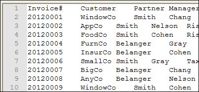
billingtextupdate01

Import the Data

In this example, the billing data was imported to Excel from the text file, onto a worksheet named BillingData. This created an external data range with a connection to the text file.

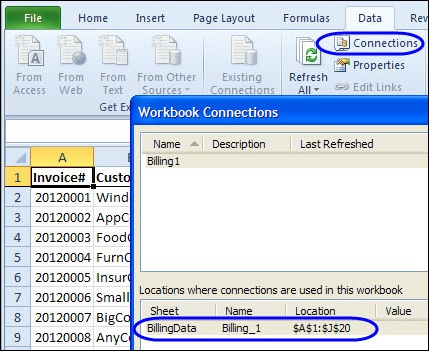
billingtextupdate02

You can create a pivot table based on the imported data, to show a summary of the billing data.

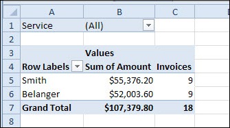
billingtextupdate03

Update the Text File

If new billing records are added to the text file, they appear in the external data range when it’s refreshed. However, you might not see the new data in the pivot table that is based on the imported data.

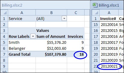
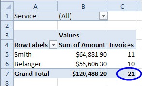
In the screen shot below, there are now 21 invoices in the imported data, but even after refreshing the pivot table, it still shows only 18 invoices. The latest data doesn’t appear in the pivot table.

billingtextupdate04

Use the External Range Name

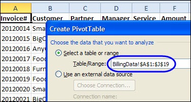
When you create a pivot table from an external data range, the default data source is a reference to a range of cells, such as BillingData!$A$1:$J$19, where the external data range is located.

billingtextupdate06

If you use the external data range’s address as the pivot table source, it does not automatically expand, if new data is added to the external data range.

However, when you import external data to an Excel worksheet, a named External Data Range is created, and if you base the pivot table on this named range, it adjusts automatically if records are added or removed.

Change the Pivot Table Source

If a pivot table is based on a specific range of cells, you can change its data source, so it uses the external data range name.

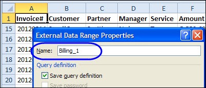
To see the name of the external data range, right-click a cell in the external data range, and then click Data Range Properties. The range name is shown at the top of the External Data Range Properties dialog box. Click OK to close the dialog box.
To base the pivot table on this range, select a cell in the pivot table, and then click the Options tab on the Ribbon.
In the Data group, click Change Data Source.
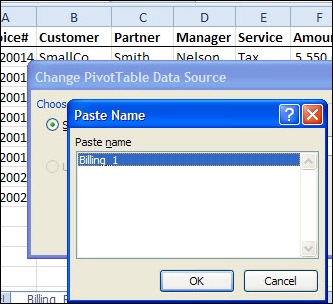
With the Table/Range highlighted, press the F3 key, and click on the external data range name, e.g. Billing_1
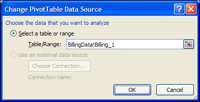
The Table/Range box will show the sheet name and the external data range name.
Click OK, to close the Change PivotTable Data Source box.

After the pivot table data source is changed to use the external data source named range, it will update automatically, if data is added or removed.

Refresh the pivot table to see the new data in the summary.

_______________________

Create Worksheet for Each Pivot Item

Last week, Angella emailed me, to ask if there was a way to create a copy of a pivot table, for each item in a report filter.

I suggested that she use a built-in pivot table feature, which is designed to do that – Show Report Filter Pages. The instructions for using this feature are shown below.

showreportfilterpages

However, this built-in feature only copies the pivot table to a new sheet – it doesn’t copy any other content from the original sheet. Angella wanted the pivot table, and she wanted all the other content too.

So, I created a macro that will copy the original sheet, name the copied sheet, and select the pivot item in the copied sheet’s pivot table. You can see the sample code on my Contextures site.

If you just need a copy of the pivot table, you can do the job quickly and easily with the Show Report Filter Pages feature.

Copy Pivot Table with Show Report Filter Pages

To create a quick copy of a pivot table, for each item in a Report Filter field, follow these steps:

Select a cell in the pivot table (the pivot table must have at lease one Report Filter)
On the Ribbon, under the PivotTable Tools tab, click the Options tab
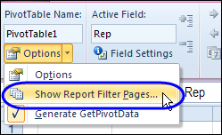
At the left, click Options, then click Show Report Filter Pages
In the Show Report Filter Pages dialog box, select one of the filters, and click OK
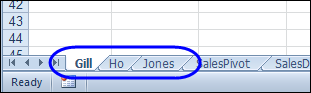
A new worksheet will be added for each* pivot item, named for the pivot item. (*see exceptions below)

Note: If a sheet with the item’s name already exists, another sheet will be added, with a number added at the end.

showreportfilterpagessheets

Report Filter Page Exceptions

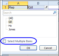
When you run the Show Report Filter Pages command, it might not create a new sheet for each item in the Report Filter. The results will be affected by

the setting for Select Multiple Items
which items are currently selected in filter

filterselectmultipleitems

Select Multiple Items Turned Off

If (All) is selected, a sheet should be created for each item.
If a specific item is selected, a sheet will not be created for that item. I guess that Excel assumes that since you already have a pivot table with that item’s data, you don’t need another one.

Select Multiple Items Turned On

If (All) is selected, a sheet should be created for each item.
If one item is selected, a sheet will be created for that item only.
If two or more items are selected (Multiple Items), a sheet will be created for each selected item.

Note: Select Multiple Items is turned off in the pivot table copies, even if it is turned on in the original pivot table.

Use VBA to Copy the Entire Worksheet

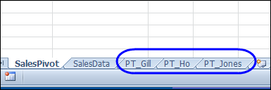
If you want to copy all the other content from the original worksheet, along with the pivot table, you can sample code on my Contextures site on my Contextures site. My code adds a “PT_” prefix to the sheets, and deletes any existing “PT_” sheets, if necessary.

pivotitemsheetsadded

___________________

Change Number Format in Pivot Chart

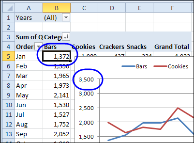
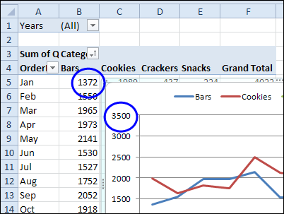
When you create a pivot chart from a pivot table, the numbers on the chart’s axis are in the same format as the pivot table’s numbers. In the screen shot below, the numbers are in General format, with no comma and no decimals.

Video: Change Pivot Chart Number Format

This short video shows how to change the number format for the pivot chart only, or change the number format for both the pivot chart and the pivot table. There are written steps below the video.

Change Pivot Table and Chart

To change the number format in both the Pivot Table and the Pivot Chart, you can change a setting in the pivot table value field. For example, if you want to add a comma separator, follow these steps

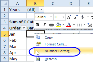
In the pivot table, right-click on a cell in the value field. In this example, the Quantity field is in the Values area.
In the popup menu, click Number Format
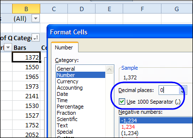
In the Format Cells dialog box, click the Number category
Change the number of decimals to 0, and add a check mark to Use 1000 Separator.
Click OK, and the number format is applied to both the pivot table and the pivot chart.

Use Different Number Format in Pivot Chart

In some cases, you might want a different number format in the pivot chart, rather than making it the same as the pivot table. In this example, you’ll format the pivot chart to show the numbers as thousands, so the numbers take less room.

Follow these steps to change the pivot chart number format, without affecting the pivot table:

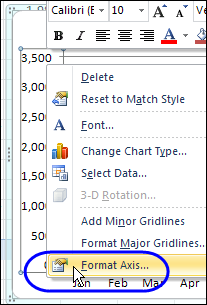
In the pivot chart, right-click a number in the axis, and then click Format Axis.
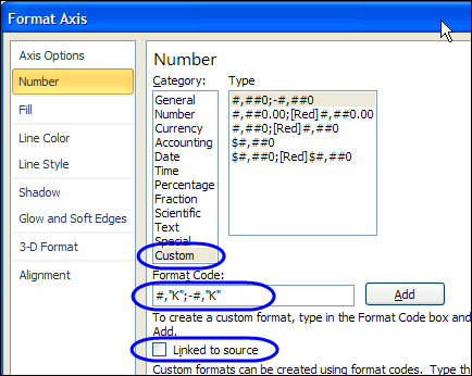
In the Format Axis dialog box, click Number, in the list at the left.
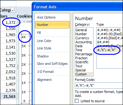
Click the Custom category. This automatically removes the check mark from Linked to Source, which disconnects the axis labels from the formatting in the pivot table.
In the Format Code box, type a code for the formatting, such as: #,”K”;-#,”K”
Click Add, to create the custom number format code, and to apply the format. Only the pivot table has changed – the pivot table numbers are sill in the previous format.
Click Close.

_________________

Calculate Differences in a Pivot Field

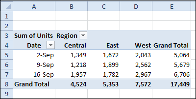
With a pivot table, you can quickly summarize data, and show the Sum or Count for thousands of records. For example, in the pivot table shown below, the weekly regional sales are shown.

differencefrom01

Besides showing a basic sum or count for the data, you can use custom calculations, to show things like a running total, or the differences between items in a pivot field.

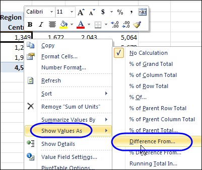
Right-click on a value cell in a pivot table, then click Show Values As, to see a list of custom calculations that you can use.

differencefrom02

Calculate the Difference

One that I use frequently is the Difference From custom calculation, that subtracts one pivot field value from another, and shows the result.

Note: If you want to show the difference between pivot fields, instead of pivot items, you can create a calculated field.

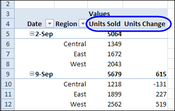
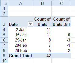
In the pivot table below, a second copy of the Units field has been added to the pivot table, and it shows the difference from the sum of one week’s sales to the next.

differencefrom05

Change the Summary Function

You can use different summary functions with a custom calculation — not just a Sum. In the example shown below, the Units field is added to the Values area twice.

Both copies of the Units field are set to show the Count summary function.
The second copy of the Units field is changed to a custom calculation for Difference From.

difference from count

Custom Calculation Tips

If you’re using custom calculations, here are a few tips to make them more effective.

To make the data easier to understand, you can change the heading from “Sum of Units” to “Units Change”.
You can add another copy of the Units field to the pivot table, and show both the total sales and difference in weekly sales
Experiment with the pivot table layout, to find the arrangement that will be easiest to read and understand.
Remember that a custom calculation can only calculate on items within the same pivot field. If you want to show the difference between pivot fields, instead of pivot items, you can create a calculated field.

Watch the Difference From Video

To see the steps for creating a Difference From custom calculation, please watch this short video tutorial.

Download the Sample File

To test the Difference From custom calculation, you can download the sample file from my Contextures website: Custom Calculations

____________________

PivotPower Premium Excel Add-in

There is a PivotPower add-in that’s available on my Contextures website, which helps with your pivot table tasks.

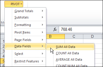
It automates some of the features that aren’t built in to an Excel pivot table, and makes some of the buried Excel pivot table features easier to access. For example, there is a command that changes all the data fields to SUM, which is handy when Excel defaults to COUNT.

pivotpowersum01

Store Favorite Settings

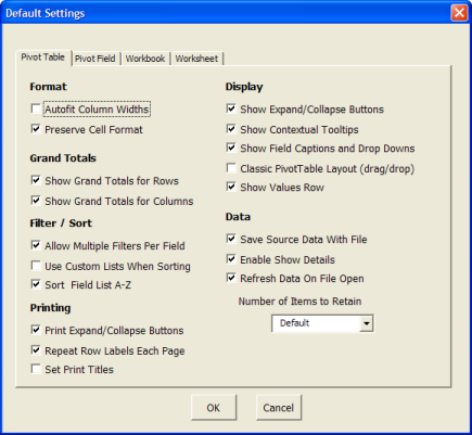
I’ve added new features to the add-in, to make it even more useful. Now you can store your favorite pivot table settings in the add-in, and then apply those settings to any pivot table, and the active sheet and workbook.

Pivot Table Default Settings

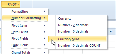
There’s a list of the new features below, and one of my favourites is Currency SUM. It changes the selected field to the SUM function, formatted as currency.

pivotpowerpremcurrencysum

Watch the PivotPower Premium Demo Video

To see a few of the new features in PivotPower Premium, you can watch this short video.

What’s New in PivotPower Premium?

The following features have been added in the new version of PivotPower Premium:

User Guide

Details on installing the add-in, and description of the commands

Formatting

Column Width Autofit On
Column Width Autofit Off

Number Formatting

Currency
Number – 2 decimals
Number – 0 decimals
Currency SUM
Number – 0 decimals COUNT

Pivot Items

Hide All (Blank) Items
Show All (Blank) Items

Pivot Fields

Clear All Fields
Field List A-Z
Field List Source Order

Grand Totals

Show All Totals and Subtotals
Hide All Totals and Subtotals

Cache

Create New Cache

Purchase the PivotPower Premium Add-in

To make your pivot table tasks easier, you can purchase the PivotPower Premium add-in, at my Contextures website.

PivotPower Premium Add-in

_______________

Show Missing Items in Excel Pivot Table

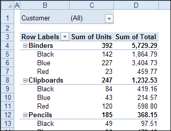
A pivot table shows a summary of the source data, and in the screen shot below you can see all the products that were sold, and the quantities for each colour.

showallpivotitems01

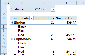
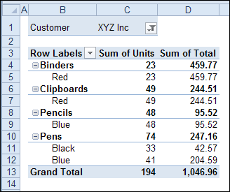
When you filter the pivot table, some of that data might disappear. For example, in the pivot table shown below, the Customer field has been filtered to show XYZ Inc. orders.

They didn’t order all the colours for each product, so the pivot table is smaller. It’s only showing the products and colours that XYZ Inc. ordered.

showallpivotitems02

Instead of having the pivot table change size, so it shows only the applicable items, you can change a field setting, to keep it consistent.

Show All Items in Excel 2010

To make all the items appear, even if the pivot table is filtered, you can change a Layout setting in the pivot table. This setting applies to a single field, so you’ll have to make the following change to each field in which you want to see all the items.

To show all items for a pivot field in Excel 2010 or 2007:

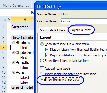
Right-click an item in the pivot table field, and click Field Settings
In the Field Settings dialog box, click the Layout & Print tab.
Check the ‘Show items with no data’ check box.
Click OK

showallpivotitems03

After the setting is changed, all the colours are listed for each product, even if they weren’t sold for the selected customer.

showallpivotitems04

To see the instructions for changing the setting in Excel 2003, please go to my Contextures website: Pivot Table Field Settings

Watch the Video

Watch this video to see the steps for changing the layout setting in Excel 2010 or 2007.

_____________________

Clear All Fields From a Pivot Table

Occasionally, you might want to tear down a pivot table, and start from scratch. You don’t have to delete the pivot table though – you can clear all the fields, and then start adding the ones you want.

Clear Pivot in Excel 2010

If you’re using Excel 2010 or 2007, it’s easy to clear the pivot table, using a Ribbon command.

Select a cell in the pivot table that you want to clear.
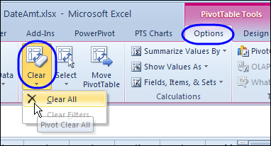
On the Ribbon, under PivotTable Tools, click the Options tab.
In the Actions group, click Clear, then click Clear All

RibbonClearAll

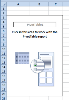
All the pivot fields are removed, and you’re left with an empty pivot table layout.

pivotempty

Undo the Clear

There’s no confirmation message when you click Clear All, so you can’t change your mind after you click that command.

However, you could click the Undo button, before performing any other actions, and all the pivot fields will be put back.

Clear the Pivot Table in Excel 2003

There’s no Clear All command in Excel 2003 and earlier versions, but you can manually remove the fields from the pivot table layout, either on the worksheet, or in the Pivot Table Wizard.

Clear the Pivot Table With Programming

The following code will clear all the fields from a pivot table, and make the field list visible, so you can start to rebuild it. Copy this code to a regular module in your workbook.

Note: You can’t undo the Clear All if you use this code. You could save the workbook before running the code, and then close without saving again, if you change your mind.

Sub ActiveCellClearPivot()
'clears pivot table for active cell
On Error Resume Next

Dim pt As PivotTable
Dim pf As PivotField

Set pt = ActiveCell.PivotTable
If Not pt Is Nothing Then

  pt.ManualUpdate = True
  
  'test version of Excel
  If CDbl(Application.VERSION) >= 12 Then
      'for Excel 2007 and later
      pt.ClearTable
  Else
    For Each pf In pt.VisibleFields
          pf.Orientation = xlHidden
    Next pf
  End If
  
  pt.ManualUpdate = False

  ActiveWorkbook.ShowPivotTableFieldList = True
End If

End Sub

_____________

Grouped and Ungrouped Dates from Same Pivot Table Source

In some workbooks, you might create two or more pivot tables that are based source data. Even if they are on different worksheets, those pivot tables will share some features, such as calculated items and grouped fields.

pivotcacheshared01

So, if you group the dates in one pivot table, the same grouping will show up in the other pivot table. This occurs because the pivot tables share the same pivot cache. You can manually create a separate pivot cache, by copying one of the pivot tables to a different workbook, temporarily. See the instructions here.

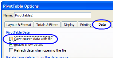
Note: If you create a separate pivot cache for one of the pivot tables, the file size might increase substantially. To reduce the effect, you can turn off the option to save the source data with the file.

pivottableoptionssavedataoff

Create New Pivot Cache with VBA

Instead of manually creating a separate pivot cache for a pivot table, you can select a cell in the pivot table, and run the following code.

It adds a temporary sheet to the workbook, and creates a new pivot table there, based on the same data source, but in a new pivot cache. The selected pivot table is set to the same pivot cache as the new table, and then the temporary sheet is deleted.

Sub SelPTNewCache()
    Dim wsTemp As Worksheet
    Dim pt As PivotTable
    
    On Error Resume Next
    Set pt = ActiveCell.PivotTable
    
    If pt Is Nothing Then
        MsgBox "Active cell is not in a pivot table"
    Else
        Set wsTemp = Worksheets.Add
        
        ActiveWorkbook.PivotCaches.Create( _
            SourceType:=xlDatabase, _
            SourceData:=pt.SourceData).CreatePivotTable _
            TableDestination:=wsTemp.Range("A3"), _
            TableName:="PivotTableTemp"
        
        pt.CacheIndex = wsTemp.PivotTables(1).CacheIndex
        
        Application.DisplayAlerts = False
        wsTemp.Delete
        Application.DisplayAlerts = True
    End If
    
exitHandler:
        Set pt = Nothing

End Sub

_____________________

Format Pivot Table Labels Based on Date Range

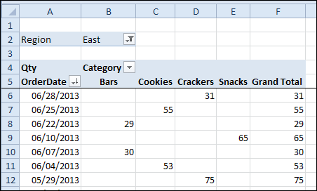
In a pivot table that contains a long list of dates, you can use conditional formatting to highlight a specific date range. In this example, the pivot table contains forecast data for 2.5 years, with dates in the OrderDate field.

pivotcondformatdates01

When the file opens, we’re usually interested in checking the forecast amounts for the upcoming month. It can take a bit of time and concentration to find those dates in the long list. We’ll highlight the labels in yellow, so they stand out, and are easy to find.

We’ll use dynamic conditional formatting (Next Month), so the highlighting will change each month when we open the workbook.

Highlight the Upcoming Month

Follow these steps to highlight Row Labels where the order forecast date is in the upcoming month. It’s currently August, so the September dates will be highlighted.

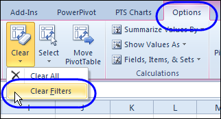
In the pivot table, remove any filters that have been applied – all the rows need to be visible before you apply the conditional formatting.

Select all the dates in the Row Labels that you want to format.
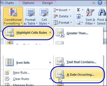
On the Ribbon, click the Home tab, and then in the Styles group, click Conditional Formatting.
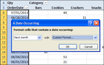
In the list of conditional formatting options, click Highlight Cells Rules, and then click A Date Occurring.

In the date range drop-down, select Next Month, and then click the arrow to open the formatting drop-down list.
Select one of the formatting options, or create a Custom Format. I selected Custom Format, and used a yellow fill colour.

Click OK to close the A Date Occurring dialog box.

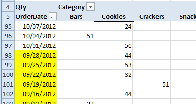
The dates from the upcoming month are highlighted, and will stand out in the report when you open the workbook.

pivotcondformatdates04

Conditional Formatting Warnings

This pivot table’s source data won’t change, because we don’t alter the forecast after it has be finalized.

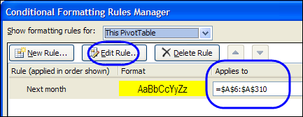
However, if you apply conditional formatting to a pivot table, and new data is added, it might not be included in the formatted area. Be sure to check the range, in the Manage Rules box for Conditional Formatting, and edit the rule, if necessary.
Also, if you change the location of the date field, the conditional formatting will not automatically move with that field. You will have to modify the conditional formatting rule, to point to the new location.

pivotcondformatdates05

___________________________-

Change Pivot Table Report Filters With VBA

With Report Filters at the top of your pivot table, you can select specific items from a field, and narrow the scope of your report.

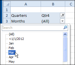
In the pivot table shown below, the order date field has been grouped, and Quarters and Months are in the Report Filter area.

reportfilterchangevba

Change Report Filters Automatically

I’ve previously posted sample code for changing one (or all) pivot table’s report filters, based on changes in another pivot table. In one of my Contextures Blog posts, Ian asked if we could change one report filter in a pivot table, based on another report filter in the same pivot table.

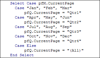
That sounded like an interesting challenge, so I’ve created code that changes the Quarters filter, when a month is selected. For example, if you select May, it will change to Qtr2. If your fiscal year is different, you could change the quarters in the code.

reportfilterchangevba02

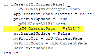
If you select a different Quarter, the Months filter will automatically change to "(All)". Then, if you want a specific month within that quarter, you could select it.

reportfilterchangevba03

Download the Sample File

To download the sample file, please visit the Pivot Tables VBA – Report Filters page on the Contextures website. The file is in Excel 2007/2010 format, zipped, and contains macros. Enable macros when you open the file, if you want to test the code.

In the file, to see the code, right-click on the pivot table sheet tab, and click View Code.

__________________