

One of the advantages of summarizing your data in a pivot table is that you can filter the results, to focus on specific items.
Author: Debra
Refer to Value Cells in GetPivotData Formula

When you type an equal sign, then click on a pivot table value cell, a GetPivotData formula is automatically created. We’ll see how to make those formula more flexible, so you can quickly change the results.
Continue reading “Refer to Value Cells in GetPivotData Formula”
Show Percent Difference in Pivot Table Amounts

With one of the built-in custom calculations in a pivot table, you can quickly show the percent difference between two amounts. In this example, forecast amounts have been entered for each product, for each month. When they become available, the actual amounts are entered in the workbook.
Continue reading “Show Percent Difference in Pivot Table Amounts”
Grouping Shows Items Before and After Date Range

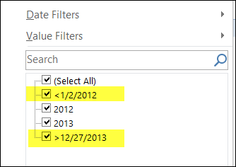
When you group a date field, Excel automatically creates creates groups for all the dates before the start date and after the end date. These items start with a “<” or a “>” symbol, such as “<2012-01-01” and “>2013-12-31”
Usually, you will only see these dates in the filter drop downs.
Continue reading “Grouping Shows Items Before and After Date Range”
Change All Number Formats in Pivot Table

Last week, I asked for your input in my survey on pivot table number formats. There were 3 questions in the survey:
- Which number format do you use most often in pivot tables?
- How many decimal places do you usually set?
- If you use Number format, do you usually include the 1000s separator?
Find MIN IF and MAX IF From Excel Pivot Table

In Excel, you can use array formulas to find MIN IF and MAX IF. For example:
- What was the lowest total order price for the Carrot Bars product?
- What was the highest price for that product?
Continue reading “Find MIN IF and MAX IF From Excel Pivot Table”
Show Zero in Empty Pivot Table Cells

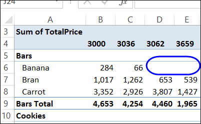
When you set up a pivot table, there might be a few blank cells in the Values area. In the example below, no Banana Bars were sold at stores 3062 or 3659.
Duplicate Items Appear in Pivot Table

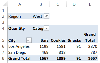
When you create a pivot table it groups the items from your data, and calculates a total for each group. In the screen shot below, you can see the total sales for each category, in each city in the West region.
Create Pivot Chart from Data in Excel 2013

With a new feature in Excel 2013, you can create a pivot chart right from the source data – you don’t have to build a pivot table first.
Continue reading “Create Pivot Chart from Data in Excel 2013”
Prevent Subtotals from Appearing

If you add more than one field to the Rows or Columns area in a pivot table, some of the fields automatically get subtotals. In the screen shot below:
- the City field has a subtotal, because it is an outer field – there is at least one field after it in the layout. Outer fields get subtotals by default.
- the Category field does not have a subtotal, because it is an inner field – there is no field after it in the layout. The innermost field in the Rows or Columns area doesn’t get a subtotal.