Pivot tables let you summarize thousands of rows of data, with just a few clicks. If you want to focus on a specific part of that summarized data, here are a couple of pivot table filter tricks.
The Excel Pivot Table Field List helps you build and modify your pivot tables quickly. But you don’t have to stick with its default settings! See how to change the Pivot Table Field List settings, so it works best for your needs.
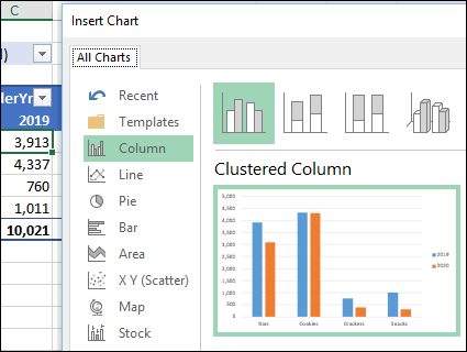
Instead of adding a static title to your Excel pivot chart, use a worksheet formula to create a dynamic chart title. When you change a pivot table filter, the chart title updates automatically, to show what you selected!
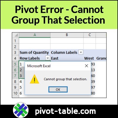
In an Excel pivot table, if you try to group a date or number field, you might see an error message. The message box shows a yellow warning label, and the text says, “Cannot group that selection”.
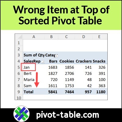
After you sort an Excel pivot table, the wrong item might appear at the top of a column. For example, in the screen shot below, the list of Sales Rep names has Jan at the top. Below that name, all the other names are sorted in the correct alphabetical order.
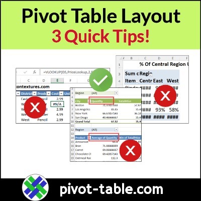
Do you ever make a quick pivot table, then spend the next 30 minutes trying to make it look good? Here are three quick pivot table layout tips, to make your job a bit easier!
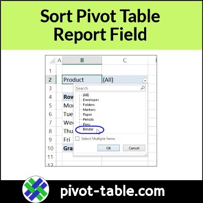
If you have a report filter at the top of your pivot table, do the items in the drop down list ever appear out of order? That happens in my pivot tables occasionally, and there isn’t a quick and easy way to fix the problem!
After you create an Excel pivot table, the source data usually changes. New records are added, and old records might be changed or deleted.
Later, when you refresh the pivot table, you should see a summary of your updated data, but sometimes there’s a problem – old data sticks in the drop down lists.
Example: Region Names Changed
To show this pivot table problem, I made short video, which you can see in the next section.
My sample file has data from a fictional sales company, and the source data was changed:
Central region was merged into the East region.
Sales records were changed from Central to East
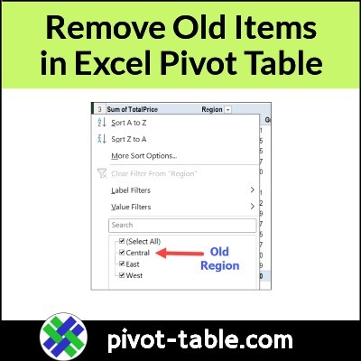
After making those changes, I refreshed the pivot table. As expected, the Central region’s name disappeared from the Region headings.
However, Central still shows up in the Region drop down.
Video: Clear Old Pivot Table Items
In this short video, I show how you can clear the old Region name from the pivot table drop down list.
Doing this will also prevent old items from appearing in this pivot table, in the future.
Video: Clear Old Items – Default Settings
In Excel 365, and Excel 2019, it’s even easier to avoid old items in pivot table drop downs.
Instead of changing this setting for every pivot table that you create, you can change it once, in your Excel default settings for Pivot Tables.
In the video below, I show the steps for changing an individual pivot table, like I did in the previous video.
Then, at the 2:57 mark, I show how to change the default setting, in Excel 365. You can skip to that section, if you’d like!
Prevent Old Items in Pivot Table
To stop old items from showing in an existing pivot table, follow the steps below.
NOTE: This setting will affect all the pivot tables that use the same pivot cache.
First, right-click a cell in the pivot table
Next, in the right-click pop-up menu, click on PivotTable options
In the PivotTable Options dialog box, click on the Data tab
In the Retain Items section, there is a drop down for “Number of items to retain per field”
By default, that is set to Automatic.
Click the drop down arrow, and select None from the drop down list.