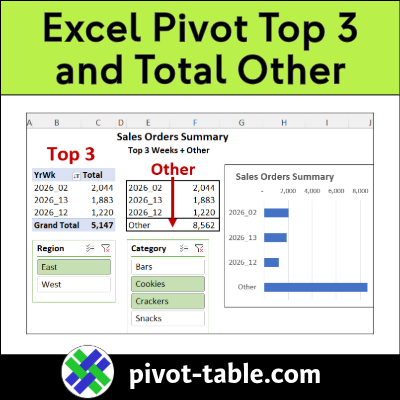
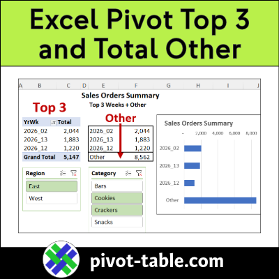
Excel Pivot Table Filter – Show Top 3 and Total Other

In a short video below, I show how to set up an Excel pivot table with the top 3 items, and a total for all the remaining items, grouped as “Other”.

Video : Pivot Top 3 and Total Other

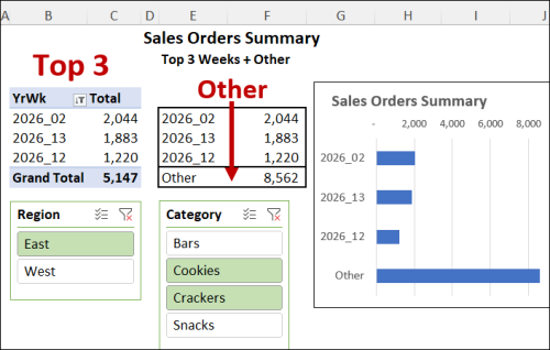
In this video, I show how to build a food sales summary in Excel.

A pivot table shows the sales for the top 3 weeks.
Sales for all the remaining weeks are grouped as “Other”.
A bar chart shows the Top 3 and the Other sales

✅ To follow along, download the Pivot Top 3 + Other (Start) Excel file. The completed version is in the Downloads section.

Building the Top 3 + Other Summary

Here’s a quick overview of how I built the food sales summary.

For detailed steps, and the completed Excel file, go to the Excel Pivot Table Top 10 Filters page on my Contextures site.

Data and Pivot Table

In the sample file, there’s sales data on the Orders sheet.

On the Summary sheet, there’s a pivot table based on the sales data.

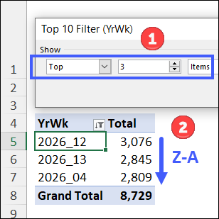
Two fields are showing in the pivot table – YrWk, and TotalPrice (Total).
YrWk field has a Top 10 filter applied, with 3 as the number of items to show
Total column is sorted in descending order, so the largest amounts are at the top.

Pivot Table Slicers

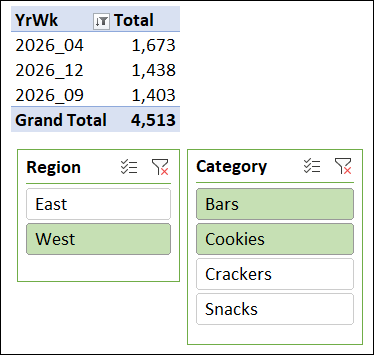
To make it easy to filter the pivot table, I selected a cell in the pivot table, and inserted Slicers for the Region and Category fields.

Pivot Table – Totals

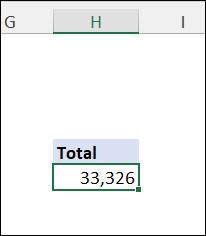
To calculate the overall totals, I copied the existing pivot table, and pasted a copy in column H

In the new pivot table, I removed the YrWk field, so only the grand total is showing.

Because it’s a copy of the first pivot table, the new pivot table was automatically connected to the two Slicers.

Add Formulas

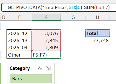
There are formulas in cells E5:F7, that pull the dates and amounts from the top 3 weeks in the pivot table.

In cell F8, a formula subtracts the top 3 total, from the overall total, using the GetPivotData function:

=GETPIVOTDATA(“TotalPrice”,$H$5) – SUM(F5:F7)

Add a Bar Chart

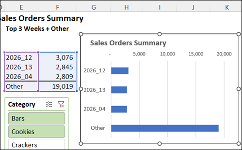
After that, I added a 2-D clustered bar chart, based on the labels and formulas in cells E5:F8.

Next, I made 3 tweaks to the chart

Moved the chart so it covers the second pivot table, which doesn’t need to be seen
Formatted the vertical axis, to put Categories in Reverse Order.
Linked the chart title to cell D1, where the worksheet heading is entered

Get the Excel File

To get the completed Excel file, and detailed written steps, go to the Excel Pivot Table Top 10 Filters page on my Contextures site. The zipped Excel file is in xlsx format, and does not contain any macros.