In Excel 2010 and later versions, you can use the % Running Total calculation, to show the current running total amount, divided by the grand total. This video shows how to analyze sales, from month to month, with the % Running Total In calculation in an Excel pivot table.
Video: Running Total Percent
Watch this short video to see how to set up the pivot table, add a % Running Total In calculation, change the row field and adjust the running total percent. To follow along with the video, you can download the sample file from my Contextures website, on the Pivot Table Running Totals page.
There are written steps below the video.
00:00 Introduction
00:19 Create the Pivot Table
01:09 Add Fields to Pivot Table
01:36 Sort by Sales Amount
01:55 Add Running Total Percent
02:44 Read the Running Total Percent
03:23 Change the Row Field
04:13 Fix the Running Total Percent
04:31 Running Total Percent by Month
04:59 Get the Sample File
Pivot Table “Show Values As”
When you add a number field to a pivot table, it usually shows up in the Values area, summarized by Sum or Count. There are many other ways to summarize the data, such as Average, Minimum and Maximum.
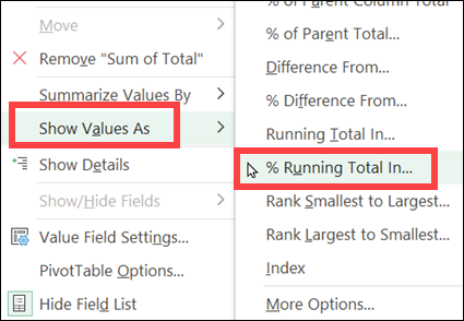
Also, there are different ways to view those Sums or Counts. Just right-click a Value field, and click “Show Values As”, to see what’s available, such as % of Column Total, or Running Total In.
In this example, we’ll analyze monthly sales with % Running Total In…
% Running Total In
When reporting on monthly sales, of my favourite “Show Values As” options is the % Running Total calculation. It shows the current running total amount, divided by the grand total. This option was added in Excel 2010.
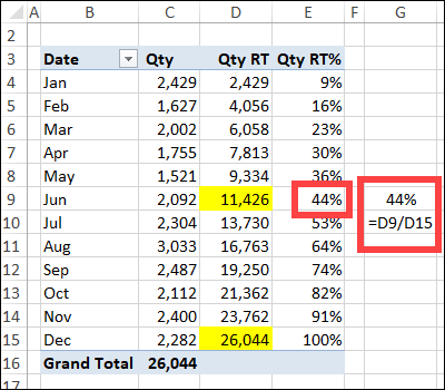
In the pivot table shown below, there are 3 Value fields in the pivot table. All 3 columns are summarizing the Sum of Qty sold in each month.
- In column C, the sum of Qty is shown, with no calculation. This is the number of units sold each month.
- In column D, the sum is shown, as a Running Total for Date. This is the total units sold, up to and including that month.
- In column E, the sum is shown, as % Running Total for Date. This is the total units sold, up to and including that month, divided by the grand total of units sold.
Poor Sales in First Half
By the end of June, 50% of the calendar year has passed. But, from the pivot table, we can see that sales were a bit low in the first 6 months of the year.
In cell D9, the pivot table shows that a running total of 11426 units have been sold, which is 44% of the overall total units sold, 26044..
To verify that calculation, I typed a formula in cell G9, to divide the June running total, by the grand total.
- =D9/D15
Fortunately, sales went better in the second half of the year. The remaining 56% of the sales occurred from July to December.
Download the Sample File
To follow along with the video, you can download the sample file from my Contextures website, on the Pivot Table Running Totals page. The file is in xlsx format, and does not contain macros.
Video: Show Running Total
If you want to show a running total in a pivot table, instead of the running total percent, watch this short video. You’ll also see how to remove the Grand Total for Rows, which is no longer needed, when the Running Total is showing.
_________________
Analyze Sales with Excel Pivot Table Running Total Percent
__________________


