If you want to prevent accidental changes to a pivot table’s layout, you can hide the pivot table buttons and labels. There are a few benefits from doing that.
Pivot Table Field Buttons
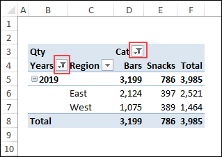
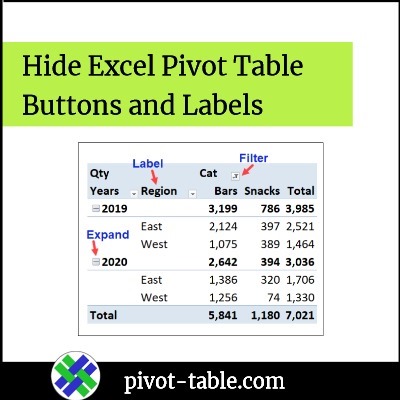
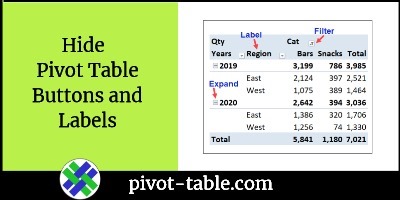
In the pivot table shown below, you can see last year’s Region sales for two food categories – Bars and Snacks.
- The Years field button has a filter symbol, and only last year’s sales are showing.
- The Cat field button also has a filter symbol, and some of the categories have been hidden.
Pivot Table Expand/Collapse Buttons
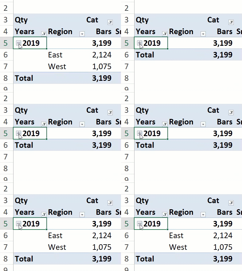
The pivot table also has an Expand/Collapse button, to the left of the Year, 2019.
- When the button shows a plus sign, click it to expand, and show the Region names for that year.
- When the button shows a minus sign, click it to collapse, and hide the Region names for that year.
Hide Excel Pivot Table Buttons
If you leave those pivot table buttons showing, it’s easy for people to change the filters that you applied, or to hide the region names (accidentally, or on purpose!).
To discourage people from changing the pivot table layout, follow these steps to make a couple of changes to the display settings.
- Right-click any cell in the pivot table
- In the pop-up menu, click PivotTable Options
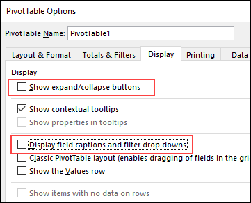
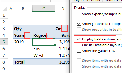
- In the PivotTable Options dialog box, click the Display tab
- To hide all of the expand/collapse buttons in the pivot table:
- Remove the check mark from the option, Show expand/collapse buttons
- To hide all of the filter buttons in the pivot table (as well as the field name labels):
- Remove the check mark from the option, Display field captions and filter drop downs
- To save your changes, click the OK button
Pivot Table With Hidden Buttons and Labels
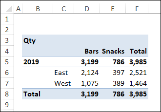
After those pivot table display options are turned off, here’s what the pivot table looks like.
Hide Filters and Show Labels
In the PivotTable Options dialog box, the filter buttons and field labels have to be turned on or off together. However, in some pivot table, you might want to hide the filter buttons, but leave the field labels showing.
To do that, use the Disable Selection macro on my Contextures website.
After running that macro:
- The pivot table still has the field labels, for Years, Region and Cat
- The filter buttons for those fields are hidden.
- In the PivotTable Options dialog box, the check mark is in the Display field captions option, so you can’t manually turn those filters on again
Benefits of Hiding Buttons and Labels
There are a few benefits of hiding pivot table buttons and labels, in some cases:
- The pivot table looks cleaner and simpler
- The filter buttons are gone, so people won’t accidentally change them
- The expand/collapse button is gone, so the region names won’t be hidden accidentally
- The field labels – Year, Region, and Cat – are hidden, and they weren’t really needed. The pivot table summary is easy to understand without those labels.
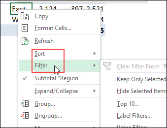
NOTE: You can still sort and filter the pivot fields, if you right-click on a cell, and use the commands in the pop-up menu.
More Pivot Table Tips
Go to my Contextures website for more tips on using the Expand/Collapse buttons and the Pivot Table Label Filters.
__________
Hide Excel Pivot Table Buttons and Labels
__________

