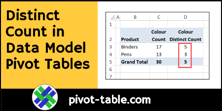
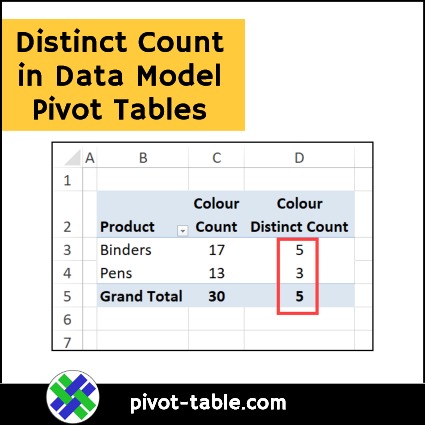
Show Distinct Count in Data Model Pivot Tables

In a pivot table you might want to see a distinct count (unique count) for some of the data, instead of an overall count.

For example, if pens and binders are sold in different colours, how many unique colours were sold for each product? Here’s how to show a distinct count in Data Model pivot tables.

Summary Functions

Pivot tables have built-in calculations, called Summary Functions. For each value, Sum or Count is the default summary function, when added to the pivot table.

Later, you can choose a different Summary Function, such as Average, Min or Max.

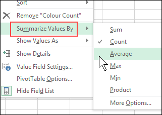
Right-click on a value cell
Point to Summarize Values By, and select one of the functions, or click More Options.

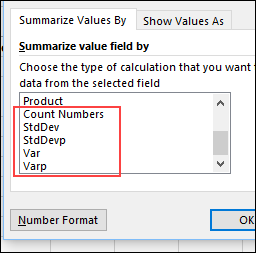
If you click More Options, a longer list of functions is shown. For a normal pivot table, the functions list ends with Var and Varp,

To learn more about the functions, visit the Pivot Table Summary Functions page on my Contextures website

Distinct Count

For normal pivot tables, you won’t see Distinct Count in the list of functions. For other ways to get a distinct count (unique count), see the Count Unique Items page.

However, a built-in Distinct Count function is available for OLAP-based pivot tables only, such as those based on the Data Model.

Video: Count Unique in Excel Pivot Table

[Update] In this short video, I show how to count unique items (distinct count) in a Microsoft Excel pivot table. This method works in Excel 2013 and later versions.

Sample Data

To show how this works, I created a Summary Function OLAP sample file that you can download.

In the sample file, there is a small table with data about office supply sales. There are 3 fields in the table – Product, Colour and Quantity.

Pivot Table – Data Model

To create a pivot table, I selected a cell in the office supply sales table, and on Excel’s Insert tab, click the Pivot Table command.

In the Create Pivot Table window, I added a check mark to the option, “Add this data to the Data Model”.

This creates an OLAP-based pivot table, instead of a normal pivot table.

List the Colours

In the pivot table, I added Product and Colour to the Rows area, and also added Colour in the Values area, as Count of Colour. This shows an overall count — how many items of each colour are in the source data.

In the Rows area, there are 5 unique colours listed under Binders, and 3 unique colours listed under Pens, but the pivot table doesn’t give us those unique counts.

Show the Distinct Count

To get a unique count of colours for each product, follow these steps:

Right-click one of the values in the Count of Colours field
Click Value Field Settings

In the Summarize Value Field By list, scroll to the bottom, and click Distinct Count, then click OK

The Colour value field changes, and the Product subtotals show a distinct count of the colours sold for each product type.

Hide the Colour Names

If you don’t need to see the colour names,

collapse the Product field, to hide the colour names (shown below)
OR, remove the Colour field from the Rows area

Get the Sample File

To download the sample file, and to learn more about the functions available, go to the Pivot Table Summary Functions page on my Contextures site.

The zipped file is in xlsx format, and does not contain any macros.

Video: Show Distinct Count in Excel 2013 With PowerPivot

To see the steps for setting up the pivot table, and creating the formula, please watch this video.

____________________