
After you create a column chart from a pivot table, you might want to change it so the chart is a combination chart type. You’d like most of the series to remain as columns, and one of the series to be a line.
In Excel 2007 there are no Combination Chart types that you can choose, as there were in the Excel 2003 Chart Wizard. However, in any version of Excel you can create your own combination charts.
In this example, the chart is a Clustered Column chart type, with the series showing the sales of each category in each city.
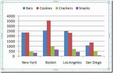
You’d like to change the Cookies series to a line, so it stands out from the other categories.
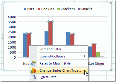
In the pivot chart, right-click on one of the Cookies columns.
In the shortcut menu that appears, click Change Series Chart Type
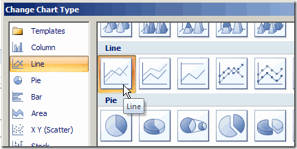
In the Change Chart Type dialog box, click the Line chart type, and click one of the Line subtypes, then click OK.
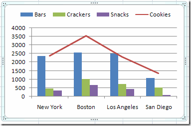
The chart is now a combination chart, with columns for Bars, Crackers and Snacks, and a line for Cookies.
___________________________
For more information on pivot tables, see the Pivot Table Topics on my Contextures web site.
___________________________
Is it possible to have a pivot chart with multiple chart types and slicers? I have a column pivot chart with one series as a line graph. When I select a new option from the slicer, the chart type for that series reverts back to the original, a column chart. Is there a way to maintain the combination pivot chart with slicers?
How do I make sure than when refreshing the combo settings are not lost? It happens every single time!
A big hug to whomever can help
Carmen