Hide Calculated Items With Zero Total

In a pivot table, you can create calculated items, in addition to the pivot items from the source data. They can create problems in your pivot table layout, such as showing cities under every region, instead of just the region in which they’re located.

In this tutorial, I’ll create a calculated item in the Category field, and then fix the problem that it creates in the City field.

Pivot Table Setup

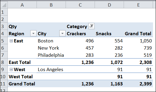
In the pivot table shown below, the Category field is in the Column headings, and it is filtered to show only two of the four categories – Crackers and Snacks.

The Region and City fields are in the Row headings, and there are 3 cities in the East and 2 cities in the West.

Create a Calculated Item

I want to add a new Category – Sweets – to show the total for the two hidden categories – Cookies and Bars.

To create the Calculated Item:

• Select one of the Category heading cells, such as cell D4.
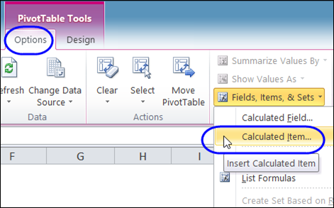
• On the Ribbon, under PivotTable Tools, click the Options tab
• In the Calculations group, click Fields, Items & Sets, and click Calculated Item

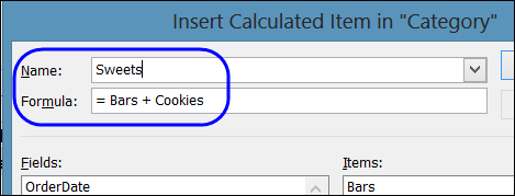
• Type a name for the calculated item – Sweets
• In the Formula box, enter the formula: =Bars + Cookies
• Click OK, to Add the new item, and to close the Calculated Item window.

Calculated Item Problems

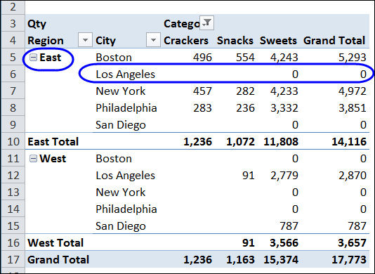
After you click OK, the Sweets category is added to the pivot table, in the Column Headings, as expected. However, each city is now listed under each region, with zero amounts in some rows.

What Went Wrong

When you add a calculated item, all the items are listed for fields that intersect the calculated item. The calculated item creates every possible combination of items in the intersecting fields, even if there is no data for that combination in the source data.

Unfortunately, you can’t change this behaviour – there’s no setting to turn it off. If possible, avoid calculated items, which can slow down a large pivot table, and create calculations in your source data instead.

Hide the Zero Rows

To hide the cities that are in the wrong region, you can use a pivot value filter to hide the rows with a zero total.

Note: This will also hide any other rows with zero grand total, so use this technique with caution.

• Right-click a cell that contains a City row label, and in the context menu, click Filter, and then click Value Filters.
• In the Value Filter window, from the first drop-down list, select Qty, which is the Values field you want to check.
• In the second drop-down list, select does not equal
• In the third box, type 0 (zero), and then click OK

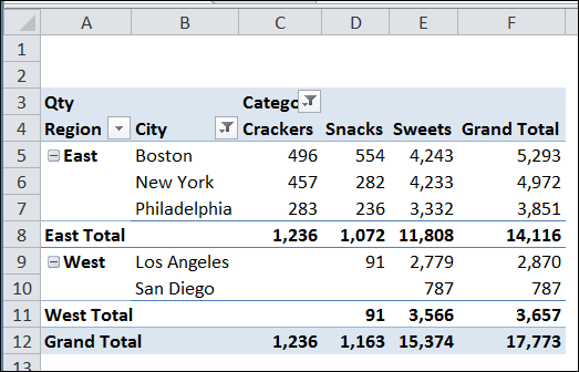
The rows where the grand total is zero are hidden, and the wayward city names disappear from each region.

_____________________