Double-clicking on a number cell in a pivot table creates a new sheet in the workbook, showing the records included in that number. Sometimes the list doesn’t look the way you’d like it to, and the numbers aren’t formatted the way they are in the source data.
For example, the source data might have sales amounts formatted as currency, or dates in a long format.
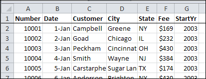
Unfortunately, those formats aren’t used in the new sheet.

You don’t have much control over the default formatting in the drilldown details list, but here are a couple of things you can do.
Change the Default Table Style
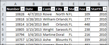
The drilldown details list is formatted as a named Excel Table, in the default style selected in the workbook. If you change the default Table Style, new lists will use the new default style.
To change the default Table Style:
- Select a cell in any Excel Table in the workbook. If there aren’t any tables, double-click a pivot table data cell, to create one.
- In the Ribbon’s Design tab, click the More drop down arrow for Table Styles
- Right-click on the style that you want as the default Table Style
- Click Set As Default
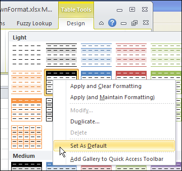
Now, when you double-click a number cell in the pivot table, the new default style is used.
Change the Normal Style
If you’re seeing strange number formatting in the drilldown details, such as dates in Currency format, the Normal Style can be adjusted.
When you select a Theme in an Excel workbook, or use the default Theme, it uses specific fonts, colours, and other format settings.
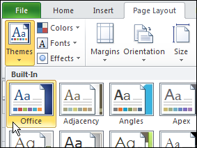
The Normal style is affected by the selected Theme, and you can make further adjustments to the Normal style. The drilldown details list will use the font and number formatting from the Normal style.
To change the Normal style:
- On the Ribbon’s Home tab, click Cell Styles
- Right-click on Normal, and click Modify
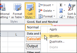
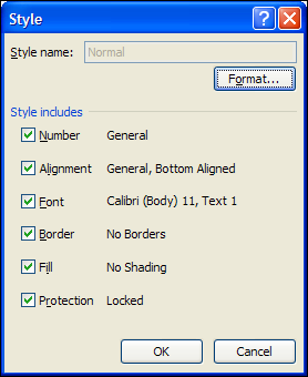
- Click the Format button, and change any of the Cell formatting options.
- Click OK, twice, to close the dialog boxes.
TIP: For number formatting, select General, so dates and numbers will look best. If you select Currency, or another specialized format, all the numbers, including dates, will get that format.
______________

Debra,
Is there any way, VBA or otherwise, to create formatting styles similar to 2007 in 2003?
Perhaps as a template, similar to “custom types” used for normal charts in 2003 when you want to save and use your own pre-formated style?
In Excel 2003 you could insert a List, and use the AutoFormat feature to add the formatting.
I’m specifically referring to Pivot Table auto formatting for 2003, which will look like the 2007 “table styles” you show in the post above.
Lists cannot overlap a range that covers a pivot tabel report, unless there’s another way.
I did find some code I can’t get to work for this problem elsewhere, but I’m not sure if I can post it here.
Is there any way we can filter the columns shown? When I double click (or select ‘Show Details’) I would get a new sheet with the data but would only see the columns I need. For example, the source data might have 8 columns but the information I want to see is in columns few of them. In my case, I have 60 columns but only 6 of them are relevent to one’s need.
EX:
Source Data =
Column1 Column2 Column3 Column4 Column5 Column6 Column7 Column8 and so on…
Ref5 Client2 AM1 1-Feb Prod1 Info1 415 $ Data1
Ref11 Client1 AM2 5-Feb Prod1 Info2 415 $ Data2
Ref14 Client4 AM1 7-Feb Prod3 Info3 552 $ Data3
Ref18 Client3 AM3 10-Feb Prod2 Info4 251 $ Data4
Ref20 Client1 AM2 10-Feb Prod3 Info5 552 $ Data5
Details sheet =
Column1 Column2 Column7
Ref5 Client2 415 $
Ref11 Client1 415 $
Ref14 Client4 552 $
Ref18 Client3 251 $
Ref20 Client1 552 $
Thanks
@DanL, no you can’t control which columns are sent to the new sheet when you double-click. All the columns from the source data will appear and you can manually or programmatically delete the ones that you don’t need.
@Debra, Thanks Debra,
I appreciate your feed back even if the answer is not the one I was hoping 😉
Dan
Anyone know how I can make the default name of a tab when drilling down on a cell in a pivot? Mine continues to change the name of the tab… Sheet 1, Sheet 2 etc. I want to make the tab name the same every time so I can run a macro with it.
Hello,
Does anyone know how to auto sort one column from the new sheet after you press drill down?
Thanks
Romina
I am wanting to drill down to the source data in a pivot table chart by double clicking the column. I entered the suggested VBA, which is working in a pivot table but not in the chart. Is there a way to drill down in a pivot chart?