Sort Pivot Table Field Left to Right

In a pivot table, you usually sort the data by the values in a column, such as the Grand Total column. By sorting, you can highlight the highest or lowest values, by moving them to the top of the pivot table.

To sort a pivot table column:

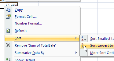
• Right-click on a value cell, and click Sort.
• Then, click Sort Smallest to Largest or Sort Largest to Smallest

Sort a Pivot Table Row

You can also sort a pivot table row by its values, left to right. This moves the largest or smallest amounts to the left of the pivot table, so you can focus on them.

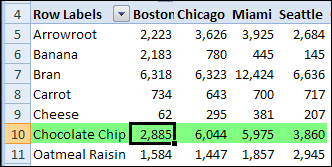
For example, in the pivot table shown below, you can sort the Chocolate Chip row, so sales per city are sorted in descending order. Currently, the cities columns are in alphabetical order, with Boston at the left.

 

To sort a pivot table row:

1. In the pivot table, right-click a value cell in the Chocolate Chip row.
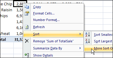
2. Click Sort, and then click More Sort Options

   
    

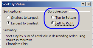
3. In the Sort By Value dialog box, under Sort Options, select Largest to Smallest.
4. Under Sort direction, select Left to Right. In the Summary section, you can see a description of the sort settings.

    

5. Click OK to close the dialog box.

View the Results

The values in the Chocolate Chip row are sorted largest to smallest, from left to right. The City column order has changed, and Chicago, which has the highest Chocolate Chip sales, is at the left.

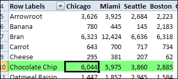
Rows for other products may not be in descending order, because the column order has been set by the values in the Chocolate Chip row.

______________