Hide Error Values in Pivot Table

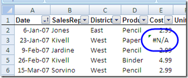
Sometimes there are errors in the source data on which a pivot table is based.

In most cases, I like to see the errors on the worksheet, so that problems are easy to spot. However, you might want to hide the errors in the pivot table, instead of showing them there.

By default, error values are displayed in a pivot table. However, by changing the PivotTable Options, you can hide the errors so blank cells appear instead of the errors:

• Right-click a cell in the pivot table
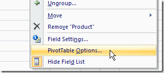
• In the context menu, click PivotTable Options.

• In the PivotTable Options dialog box, click the Layout & Format tab.
• In the Format section, add a check mark to For Error Values, Show.
• Leave the text box blank, and the errors will be replaced with blank cells. Note: You could type other characters, such as a hyphen, in the text box, to replace the error values with that character.

• Click OK to close the dialog box.

Note: This setting only affects cells in the Values area of the pivot table. If error values appear in the Row Labels, Column Labels, or Report Filter area, they won’t be replaced.

_____________________