
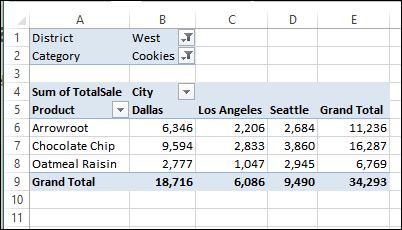
When you create a pivot table, the items in each field are sorted alphabetically, in ascending order, like the products and cities shown below.
by contextures.com

When you create a pivot table, the items in each field are sorted alphabetically, in ascending order, like the products and cities shown below.
Instead of looking at all the data in a pivot table, you can use filters to narrow your focus. See how to apply one filter, or apply multiple filters on a pivot field, without clearing the other filters.
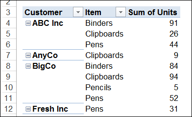
A pivot table is a great way to see a summary of sales to your customers. You can see how much they bought, and how much they spent, on each product. In the pivot table below, each customer is listed, and below the customer name is a list of products and quantities.
Continue reading “Pivot Table Shows Customers With No Purchases”
In the source data for your pivot table, you can use the drop down filters in the heading cells, to show only the records for a specific date range.
For example, in the table shown below, you could show just the orders that were shipped this week.
Continue reading “Dynamic Date Range Filters in Pivot Table”
When you add new items to a pivot table, they might not appear in alphabetical order. In the screen shot below, Binders is a new item, and it’s at the end of the list, instead of at the top.
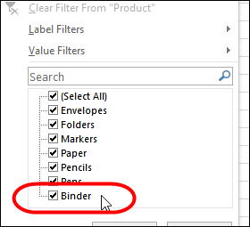
Continue reading “Show New Pivot Table Items in Alphabetical Order”
If you frequently use filters in your pivot tables, here is a quick way to clear them. Thanks to AlexJ, who shared this tip. You can find more of AlexJ’s Excel sample files on my Contextures site.
Last year, I described how to create a unique count in an Excel 2010 pivot table, by using the PowerPivot add-in. In that version, you can right-click on the table name in the field list, to add a new measure.
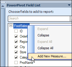
Continue reading “Count Unique Items in Pivot Table With Excel 2013 PowerPivot”
When you create a pivot table from your source data, it only shows the items that have data. For example, if you put Customers and Products in the Row area, it only lists the items that each customer has bought.
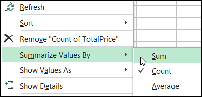
When you create a pivot table, Excel automatically makes the value fields either a SUM or a COUNT, depending on the type of data in that field. You’re not stuck with that function though — if you don’t like the summary function that Excel selected, you can change it.
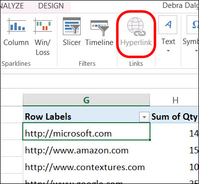
Unfortunately, you can’t add hyperlinks to a pivot table, even if there are hyperlinks in the pivot table’s source data. In the screen shot below, the Hyperlink command is not available, because a pivot table cell is selected.
Continue reading “Create Fake Hyperlinks in Excel Pivot Table”








