Sorting Pivot Table Report Fields

To focus on specific data in an Excel pivot table, you can add a field to the Report Filter area. Then, select one or more items from that pivot table field, to see the summarized data.

If you put a date field in the Report Filter area, there might be a long list of dates in the dropdown list. When you create the pivot table, the dates are usually in ascending order, with the oldest dates at the top of the list.

That’s not too convenient, if you want to focus on the latest data, instead of the oldest. How can you change the sort order, to put the newest dates at the top of the list?

Sort the Report Filter Field

Usually, it’s easy to sort a pivot table field. For example, if you right-click on a field in the Row area, the popup menu shows sorting and grouping options.
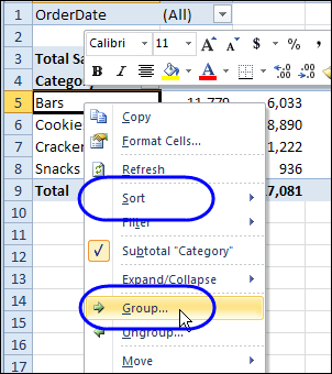
PivotFilterGroup01

However, when you right-click a Report Filter field, those sorting and grouping options aren’t listed in the popup menu.
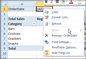
PivotFilterGroup02

Move the Pivot Table Field

To solve the sorting problem, you can use a workaround – temporarily move the Report Filter field to the Row Labels area.
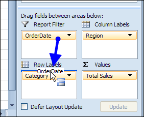
PivotFilterGroup03

Then, use the right-click popup menu to sort the date field in descending order.
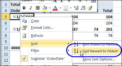
PivotFilterGroup04

Drag the field back to the Report Filter area, after you sort it.
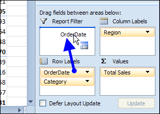
PivotFilterGroup05

Report Filter Dates in Descending Order

After you sort the field in descending order, you’ll see the latest dates at the top of the drop down list.
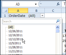
PivotFilterGroup06

It’s not the ideal solution, but it works! Maybe in the next version of Excel you’ll be able to sort the fields, without moving them from the Report Filter area.

Video: Sort Report Filter Field

Watch this very short video, to see how to show the items alphabetically, by temporarily moving the Report Filter field to the Rows area in the pivot table.

Download the Sample File

To download the sample file, please visit the Pivot Table Sorting page on my Contextures website.

_________

Include New items in Pivot Table Filter

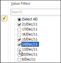
In a pivot table, you can apply a manual filter to a pivot field, by using the check boxes in the field’s drop down list.

PivotManualFilter01

In this example, there is a date field in the Row Labels area and a few dates have been selected in the manual filter.

Updating the Pivot Table Data

If you add new records in the pivot table’s source data, new dates might be added. When you update the pivot table, the new dates might appear, even if you hadn’t selected those dates in the manual filter.

Seeing the new dates could be helpful, if you want to make sure that you notice new records when they’re added. You can manually deselect the new items after they appear.

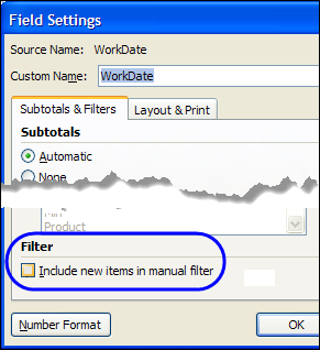
However, if you want to prevent the new dates from automatically appearing, you can change a setting in the pivot field, to specify if new items are included or not, when the field is manually filtered.

Change the Pivot Field Setting

To change the setting, and prevent new items from being included, follow these steps:

  1. In the pivot table, right-click a cell in the date field, and click Field Settings.
  2. On the Subtotals & Filters tab, in the Filter section, remove the check mark from Include New Items In Manual Filter
  3. Click OK.

PivotManualFilter02

____________

Highlight Pivot Filters With Markers

One of the benefits of using an Excel pivot table to analyze your data, is that you can use filters to focus on a specific part of the summarized results. Hiding some of the data with filters can be misleading though, if you can’t tell that filters have been applied.

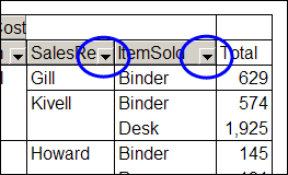
If you apply a filter in Excel 2007 or Excel 2010, the filter drop down changes to a funnel, with a tiny arrow. In the screen shot below, the ItemSold field has been filtered, to hide some of the items.

pivotfiltermarkers00

In Excel 2003, and earlier versions, if you apply a filter to a pivot field, the drop down arrow doesn’t change. The same filter was applied in Excel 2003, in the screenshot below, but both drop down arrows are the same.

pivotfiltermarkers02

Create Your Own Filter Markers

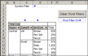
If you’d like to make it easier to tell which fields are filtered, you can use the Excel VBA code created by AlexJ, which displays a bright blue marker above each filtered field.

pivotfiltermarkers

Download the Sample File

To test the pivot table filter markers, and see the VBA code, you can download AlexJ’s sample file from the Contextures website. On the AlexJ Sample Files page, go to the Pivot Tables section, and look for:  PT0000 – Pivot Table Filter Markers

__________


Apply Multiple Filters to Pivot Table Field

A powerful feature of pivot tables is that you can filter a pivot field, to see specific results. However, if you apply a different filter to that pivot field, the first filter is removed. For example, if you filter a Row field for region names starting with “East”, and then add a Top 10 filter, the “East” filter is removed.

Use the technique shown in this video to apply multiple pivot table filters at the same time. You can use a Label filter, Value filter and Manual filter simultaneously, to fine tune your pivot table reports.

__________

Quickly Hide Selected Items in Excel Pivot Table

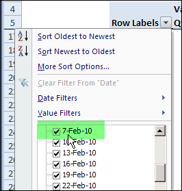
In an Excel pivot table, you might want to hide one or more of the items in a Row field or Column field. To do that, you can click the drop down arrow for the Row or Column Labels, then remove the check mark for items you want to remove.

For example, to hide the data for 7-Feb-10, you’d click on the check mark to remove it.

pivothidesel01

A Quick Method to Hide Items

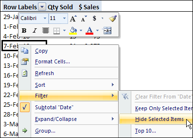
Instead of searching through a long list of items in a drop down list, you can use a quick command to hide the selected items.

  1. Right-click on an item in the Row Labels or Column Labels
  2. In the pop-up menu, click Filter, then click Hide Selected Items.
  3. The item is immediately hidden in the pivot table.

pivothidesel02

Quickly Hide All But a Few Items

You can use a similar technique to hide most of the items in the Row Labels or Column Labels.

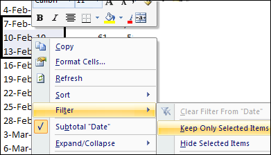
  1. Select the pivot table items that you want to keep visible
  2. Right-click on one of the selected items
  3. In the pop-up menu, click Filter, then click Keep Only Selected Items.
  4. All but the selected items are immediately hidden in the pivot table.

pivothidesel03

Watch the Pivot Table Tutorial Video

To see the steps for quickly hiding or keeping the selected items in an Excel 2007 Pivot Table, you can watch this short video tutorial.

____________

Sort Pivot Table Field Left to Right

In a pivot table, you usually sort the data by the values in a column, such as the Grand Total column. By sorting, you can highlight the highest or lowest values, by moving them to the top of the pivot table.

To sort a pivot table column:

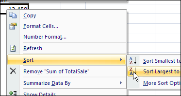
  • Right-click on a value cell, and click Sort.
  • Then, click Sort Smallest to Largest or Sort Largest to Smallest

pivotsortrow01

Sort a Pivot Table Row

You can also sort a pivot table row by its values, left to right. This moves the largest or smallest amounts to the left of the pivot table, so you can focus on them.

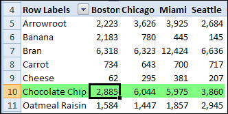
For example, in the pivot table shown below, you can sort the Chocolate Chip row, so sales per city are sorted in descending order. Currently, the cities columns are in alphabetical order, with Boston at the left.

pivotsortrow00 

To sort a pivot table row:

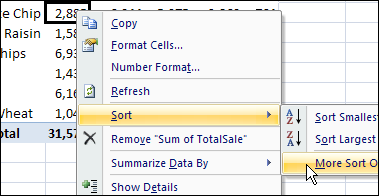
  1. In the pivot table, right-click a value cell in the Chocolate Chip row.
  2. Click Sort, and then click More Sort Options

    pivotsortrow02
     

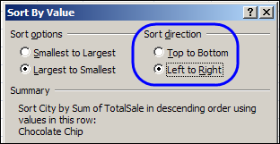
  3. In the Sort By Value dialog box, under Sort Options, select Largest to Smallest.
  4. Under Sort direction, select Left to Right. In the Summary section, you can see a description of the sort settings.

    pivotsortrow03 

  5. Click OK to close the dialog box.

View the Results

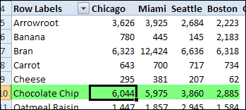
The values in the Chocolate Chip row are sorted largest to smallest, from left to right. The City column order has changed, and Chicago, which has the highest Chocolate Chip sales, is at the left.

pivotsortrow04

Rows for other products may not be in descending order, because the column order has been set by the values in the Chocolate Chip row.

______________

Excel Pivot Table Filters for Top 10

With Excel Pivot Table filters, you can limit the results to a specific part of your data. For example, you can view only the sales from the previous month, or see the products with more than $500 in sales.

If you’re interested in analyzing the best or worst results in your data, use the Top 10 filter feature in a pivot table. Although it’s called “Top 10”, you can see the Top or Bottom Items by value. You can also choose to see the values that make up a specific Percent of the total,  or the products that add up to a specific SUM.

For written instructions for this Excel pivot tables feature, see Excel Pivot Table Filters – Top 10.

To see the steps in action, watch this short Excel video tutorial for the Top 10 Filter feature.

___________

Pivot Table Date Filters

If there’s a date field in your Excel pivot table, you can use it to focus on a specific date, or a selected date range. To filter the dates, you can use the following filter types:

  • Date checkboxes
  • Date range entry
  • Dynamic date range selection

Using Date Checkboxes

If a date field is in the Row Labels area of the pivot table, do the following to show or hide specific dates.

  1. Click the drop down arrow on the Row Labels heading
  2. Select the Field name from the drop down list of Row Labels fields
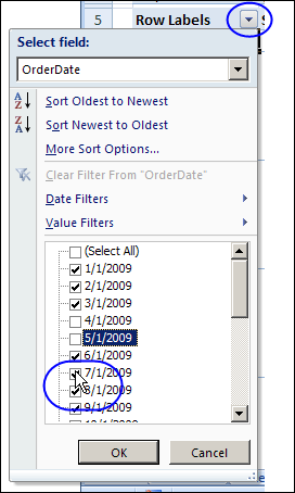
  3. In the list of dates, add check marks to show dates, or remove check marks to hide dates.
  4. Click OK

DateFilter02

Clear a Date Filter

To remove a date filter from a pivot table field:

  1. Click the drop down arrow on the Row Labels heading
  2. Select the Field name from the drop down list of Row Labels fields
  3. Click Clear Filter From [date field name]

Filter for a Specific Date Range

If a date field is in the Row Labels area of the pivot table, do the following to show a specific date range.

  1. Click the drop down arrow on the Row Labels heading
  2. Select the Field name from the drop down list of Row Labels fields
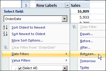
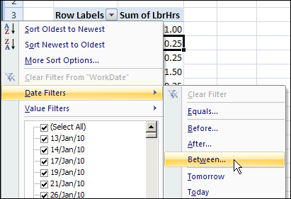
  3. Click Date Filters, then click Between..
    • .DateFilter03
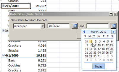
  4. In the Between dialog box, type a start and end date, or select them from the pop up calendars.
  5. Click OK.

DateFilter04

Filter for a Dynamic Date Range

A Dynamic Date Range is one that changes automatically, as time moves forward. For example, Tomorrow, which will represent a different date, every day that you open the pivot table file.

If a date field is in the Row Labels area of the pivot table, do the following to show data from the current month, as a dynamic date range.

  1. Click the drop down arrow on the Row Labels heading
  2. Select the Field name from the drop down list of Row Labels fields
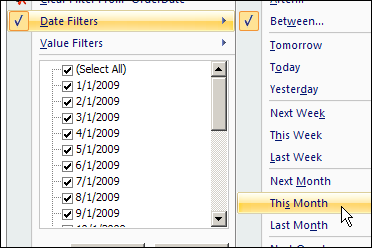
  3. Click Date Filters, then click This Month

DateFilter05

Date Filters in the Pivot Table Report Filters

Unfortunately, the Date Range filters and Dynamic Date filters aren’t available in the Pivot Table Report Filters area. If you move a date field to the Report Filters area, only the Checkbox filter type is available.

If you move a filtered date field from the Row Labels area to the Report Filters area, any filtering will be discarded, unless the check boxes were used to select specific dates.

Watch the Pivot Table Date Filters Video

To see the steps in action, please watch this short video on Pivot Table Date Filters.

______________

For more information on Pivot Tables, please see the Pivot Table Tutorials on the Contextures Website.

______________

Filter a Pivot Table for Nonconsecutive Dates

In an Excel 2007 pivot table, you can filter a date field by using the Date Filters option in the Row Labels drop down. For example, you can select all the dates between two specific dates, or filter for a dynamic range, such as Last Week.

DateFilter01 

However, when you use the row label date filters, you can only select a consecutive date range, or one specific date. You can’t select two or more nonconsecutive dates.

For example, in the screen shot above, the Work Date field is in the Row Labels area, and Labor Hours (Sum of LbrHrs) is in the Values area. In the Work Date field, you can’t use the Date Filters option to select to select January 13th, 17th and 21st.

Manually Select the Dates

Instead of using the date filter options, you can manually select items in the Row Labels drop down list. To manually filter dates in the Row Labels filter list, follow these steps:

  1. In the pivot table, click the arrow on the Row Labels heading.
  2. In the list of dates, remove the check mark from Select All, to remove all the check marks from the list.
  3. Add check marks to the dates you want to see, and then click OK.

The pivot table now shows results for work done on the selected dates, and you can focus on that data.

______________

For more information on Pivot Tables, please see the Pivot Table Tutorials on the Contextures Website.

______________

New Pivot Items Out of Order

If you add new products to your pivot table source data, and refresh the pivot table, the new products will appear in the drop down lists. Sometimes though, the new items appear at the end of the list, instead of in alphabetical order. This problem can occur if you have manually rearranged the items in the Row Labels area.

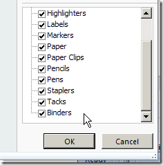
For example, binders were just added to this pivot table’s source data. When the pivot table was refreshed, Binders appeared at the bottom of the Product list, instead of the top.

ListManualSort

Because it’s not in alphabetical order, it’s difficult to find the new product in the list. You’d like the product list sorted alphabetically.

Sort the List

If a field is set for Manual sort, new items will appear at the end of the drop-down list. Follow these steps to sort the field in ascending order:

  1. Right-click a cell in the Product field. For example, right-click the Envelopes cell.
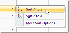
  2. Click Sort, and then click Sort A to Z.

SortAZ

When you sort the Product field, its sort setting changes from Manual to Sort Ascending or Sort Descending. This also sorts the drop-down list, and makes it easier for users to find the items they need.

______________

For more information on Pivot Tables, please see the Pivot Table Tutorials on the Contextures Website. _________________