Refer to Value Cells in GetPivotData Formula

When you type an equal sign, then click on a pivot table value cell, a GetPivotData formula is automatically created. We’ll see how to make those formula more flexible, so you can quickly change the results.

For example, in the screen shot below, I typed an equal sign in cell A1, then clicked on the Arrowroot total price in the pivot table.

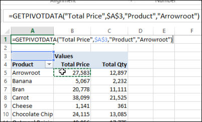
Excel created a GetPivotData formula, and shows “Total Price” as the first argument:

=GETPIVOTDATA(“Total Price”,$A$3,”Product”,”Arrowroot”)

Change Text to Cell References

To make the formula flexible, we can change the text strings to cell references, and you can see sample formulas here.

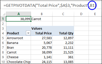
For example, type Arrowroot in cell B1, then change the formula so it refers to that cell for the product name.

=GETPIVOTDATA(“Total Price”,$A$3,”Product”,B1)

Then, you can change cell B1 to a different product, and the formula result changes automatically. Now we can see the total price for Carrot in cell A1.

Problem with Value Cell Reference

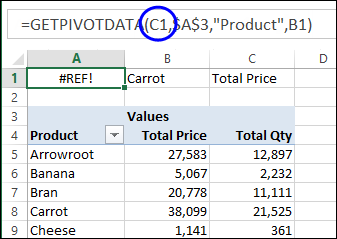
Cell references work well with the row fields, but if you try to use the same technique with the Value field name – Total Price – the formula returns a #REF! error.

In the screen shot below, I entered Total Price in cell C1, and referred to that cell. The formula returns a #REF! error, even though cell C1 contains the correctly typed field name, “Total Price”.

=GETPIVOTDATA(C1,$A$3,”Product”,B1)

Fix the Value Field Cell Reference

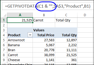
If you want to use a cell reference for a value field, use the & operator to concatenate an empty string at the start or end of the reference.

In this example, you could use

=GETPIVOTDATA(C1 & “”,$A$3,”Product”,B1)

or

=GETPIVOTDATA(“” & C1,$A$3,”Product”,B1)

The formula shows the correct total for Total Price.

Then, I can change the Value field name in cell C1 to Total Qty, and it will show that amount.

_____________________