There’s no setting that lets you show the grand totals at the top of an Excel pivot table. But watch my short video below, to see a quick trick, to get around that limitation!

Video: Show Excel Pivot Table Grand Totals at Top
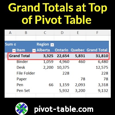
In this short video, I show the steps for creating a grand total at the top of the pivot table, and the full transcript is below the video.
- ✅ To follow along, get the Excel sample file on my Contextures site.
5 Main Steps – Grand Totals at Top
Here’s a quick summary of the 5 main steps that I shows in the video:
- Add a new column in the pivot table source data, with the heading “GT”
- Add a formula in that column, to show text in each row: =”Grand Total”
- Refresh the pivot table, then add the new field, at the top of the row area
- Change that field’s settings, to Show all Subtotals at Top of Group
- Hide the original grand totals, at the bottom of the pivot table.
You can get the Excel file, and detailed written steps, on my Contextures site.

Get the Excel File
- You can get the Excel file, and detailed written steps, on my Contextures site.
Video Transcript
Here is the full transcript for the Grand Totals at Top of Pivot Table video.
________
When you make an Excel pivot table, it will show grand totals across the bottom and down the right hand side, but it won’t let you move those to the top.
I’m going to show you a way to do that. This is Debra Dalgleish from contextures.com.
Built-In Settings
First, I’ll show you the settings that are built in.
- I’ve got a cell selected in the pivot table.
- So, it’s showing two pivot table menus up here.
- I’ll go to design and there’s grand total menu and subtotals.
- For subtotals, it will say don’t show them or show them at the bottom or top.
- But for grand totals, it just lets you pick rows or columns or both or none.
- So, we can’t use anything built in.
Create a New Field
What we’re going to do instead is create a subtotal and then show it at the top.
- I’m going to the source data for this pivot table and I’m going to add a new field and use it to show the words grand total.
- So, I’ll right-click at the top and insert.
- The new field could go anywhere.
- I just picked a spot here.
- It comes up with a default title, and I’m going to change that to GT for grand total.
I want every row to say grand total.
- So, instead of typing it and copying it down, I’ll use a formula that will automatically fill it in each row.
- equals and then in double quotes grand total.
- And when I press Enter, it just fills all the way down.
Show the New Field
Now I’m going back to the pivot table.
- Here’s the field list where we can see all the fields.
- And grand total isn’t showing up yet.
- I’ll refresh – just right-click and refresh.
And now we can see that GT field.
- I’m going to drag it where I want it in this layout above item and drop.
- So I can see grand total at the top, but it’s not showing any totals yet because it’s a subtotal.
- We’ll go and change that subtotal command.
- So design subtotals and show all subtotals at top of group.
So now we can see they’re the same as the existing official grand totals.
- I’ll just turn that off by right-clicking and removing the grand total.
__________
Show Excel Pivot Table Grand Totals at Top-Video Steps

__________