Make Pivot Chart Title Change with Filters

Instead of adding a static title to your Excel pivot chart, use a worksheet formula to create a dynamic chart title. When you change a pivot table filter, the chart title updates automatically, to show what you selected!

Video: Dynamic Pivot Chart Title

In this video, I show how to set up a dynamic title for a pivot chart. Instead of a generic title, you can have a detailed title, that includes the sales region name. And the title updates every time you change the pivot table filter!

Step 1: Get Your Pivot Table Ready

The first step is to make a pivot table. The pivot chart will be based on this table, so it’s important to set it up first.

In my example, I’ve got sales data, by food category, for two years.

There’s a region filter at the top, for the four regions: East, West, North, and South.

Note: In the Region filter, I checked the box “Select Multiple Items”, so you can pick any number of regions at once.

Step 2: Insert a Pivot Chart

Next, follow these steps to make the pivot chart:

Click anywhere inside your pivot table.
Go to the Insert tab on the ribbon.
Select Recommended Charts.
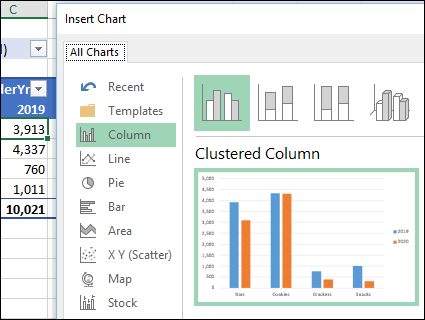
Pick the Clustered Column chart.
Click OK to add the chart.
Move or resize the chart to fit your worksheet layout.

Step 3: Add a Chart Title

Next, follow the steps below, to set up the default chart title:

Click on your chart.
Go to Design (or Chart Design) on the Excel Ribbon.
Click Add Chart Element > Chart Title > Centered Overlay.
(Optional) Point to the title box border, and drag the title where you want it.

Step 4: Check the Filter

The dynamic chart title will be based on what’s selected in the region filter, which is in cell C2 on the worksheet.

There are 3 main variations on what that filter cell could say:

All – if no filter is used
West – Or another region name, if only one region is picked
Multiple Items – if more than one region is selected

In the next step, I’ll use that filter cell in a formula next.

Step 5: Build Formula for Chart Title

Excel won’t accept a formula directly in the chart title, so I’ll make a worksheet formula, with the title text the I need.

To create the chart title’s text, I put a formula in cell G1

I used that cell because it’s easy to find, but doesn’t clutter up the worksheet.

Here’s the formula, and it refers to the region filter, in cell C2

=”Annual Sales ” & IF(C2=”All”, “All Regions”, IF(C2=”Multiple Items”, “Multiple Regions”, C2))

The formula result will start with “Annual Sales ” (there’s a space character at the end)

After that, the IF function adds text based on what’s selected in the filter cell – “All” or “Multiple Items”, or a specific region name

Step 6: Link Chart Title to Formula

The final step is to link the pivot chart title to the formula cell.

Click on the chart title once, to select it.
- Note: Don’t click inside the chart title, just on the border
Next, click in the formula bar and type =G1
Press Enter, to complete the link.

Now the chart title is dynamic, and updates on its own, every time the Region filter changes.

Step 7: Test the Title

To make sure the dynamic title is working correctly, make a few changes to the region filter, and see what happens to the chart title:

Select All – the title should say “Annual Sales All Regions”
Select Central– the title should change to “Annual Sales Central”
Select two or more regions – the title should say “Annual Sales Multiple Regions”

Chart Title Tips

Formula Cell: Keep the formula cell in view, so you can check or change it easily. Or, move it to a different location, to prevent people from changing the formula!

Add a Slicer: You could also add a Pivot Table Slicer for the Region field, so it’s easy for people to select a region. Be sure to leave the Region field in the Report Filter area too, so the chart title formula can get the information from that cell.

Get the Sample File

To get the Excel sample file for this video, go to the Excel Pivot Charts page on my Contextures site.

The zipped Excel file is in xlsx format, and does not contain any macros.

‘——————————-