You can group the dates in a pivot table in different increments, such as by year and quarter.
However, the grouping options are based on the calendar year, and there are no options for grouping pivot table dates by fiscal year. If you want to group the dates by your company’s fiscal year, which starts in July, there’s no built-in way to do that.

Fiscal Year Workaround
Because there’s no built-in option to group pivot table dates by fiscal year, you’ll have to use a workaround solution. In the pivot table source data, you can add a column with a formula that calculates the fiscal year, and then add that field to the pivot table.
For example, if your fiscal year starts in July, use the following formula to calculate the fiscal year, where the date is in cell A2:
=YEAR(A2)+(MONTH(A2)>=7)
The formula calculates the year of the date in cell A2. Then, it calculates the month of the date in cell A2, and checks to see if the month number is 7 or higher. If the month is less than 7, then zero will be added to the year, otherwise 1 will be added.
In the screenshot below, you can see the fiscal year formula for dates in June and July.
- The year for all the dates is 2010.
- For the June dates, the month is 6, which is less than 7. So, zero is added to the year, and the fiscal year is 2010.
- For the July dates, the month is 7, so 1 is added to the year, and the fiscal year is 2011.

Fiscal Quarter Workaround
If you also want to group the pivot table dates by the fiscal quarter, you can add another column to the pivot table source data. Use this formula to calculate the fiscal quarter, if the fiscal year starts in July.
=CHOOSE(MONTH(A2),3,3,3,4,4,4,1,1,1,2,2,2)
The Choose formula calculates the month of the date in cell A2. Based on the month number, the formula selects the appropriate fiscal quarter number from the numbers that follow. For example, if the month is June, the month number is 6. In the Choose formula, the sixth number is 4, so June is in fiscal quarter 4.
In the screenshot below, you can see the fiscal quarter formula for dates in June and July.
- For the June dates, the month is 6, and the sixth month in the Choose formula is 4, so June is in fiscal quarter 4.
- For the July dates, the month is 7, and the seventh month in the Choose formula is 1, so July is in fiscal quarter 1.

Add the Fiscal Dates to the Pivot Table
If you had grouped year and quarter dates in the pivot table, ungroup them and remove them.
Refresh the pivot table, and add the fiscal year and fiscal quarter fields to the Row Labels area.

Videos: Pivot Table Grouping
Learn more about pivot table grouping, and get a workbook with sample file that you can use for testing. Go to the How to Group Pivot Table Data page on my Contextures website.
First, this video shows how to group Text items in a pivot table.
Next, this short video shows the basics of pivot table grouping
______________
When you add a date field to your Pivot Table, Excel automatically groups the dates into a hierarchy, such as years and months. See how to stop pivot table date grouping in the latest versions of Excel, and a couple of workarounds for Excel 2016. You can also read about why this feature was added, and watch a date grouping video.
Prevent Date Grouping
It’s easy to prevent automatic date grouping for pivot tables in Excel 2019/365, by changing a setting. See the simple steps below.
For Excel 2016, it takes more work — use either the Excel 2016 Workaround, or the Excel 2016 Registry tweak, described below.
Further down in this blog post, you can read more about date grouping in Filters, and the benefit of pivot table date grouping, which started in Excel 2016.
Excel 2019/365 Setting
If you’re using Excel 2019 or Excel for Office 365, there’s good news. You don’t have to use workarounds or make changes to the registry. Now, you can simply change one of the Excel options, to stop pivot table date grouping.
NOTE: This is an application-level setting, not a setting for individual workbooks.
To turn this setting off:
- At the top of Excel, click the File tab
- Click Options, then click the Data category
- In the “Data options” section, add a check mark to “Disable automatic grouping of Date/Time columns in PivotTables”
- Click OK to close Excel Options

Excel 2016 Workaround
In Excel 2016, there isn’t an easy way turn off pivot table date grouping. However, to prevent dates from automatically grouping in Excel 2016, you can use this 2-step workaround:
- Add the date field to the pivot table Report Filter area first. Dates are not automatically grouped there
- Then, in the PivotTable Fields list, drag the date field into the Rows or Columns area. Dates will remain ungrouped.

Excel 2016 Registry
The only way to turn off pivot table date grouping in Excel 2016, if you’re brave enough, is by making a change to the Windows Registry.
To do that, follow the instructions in this article by Microsoft’s Excel team. Remember to make a backup of the registry first, and read the warning at the top of that page.
Date Grouping in Filters
Starting in Excel 2007, dates have been automatically grouped into a hierarchy, such as years and months, when you turn on an AutoFilter or create a named Excel table.
You can change an Excel option to turn that automatic grouping on or off, and there are instructions and a video on my Contextures website.

Date Grouping in Pivot Tables
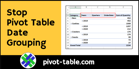
Pivot Tables dates weren’t grouped in earlier versions of Excel, but that behaviour changed in Excel 2016. Since that version, dates in Pivot tables have been automatically grouped too.
Here’s a pivot table in which I added the Category and OrderDate fields to the Rows area. Because of the date grouping, extra columns were automatically created, to show the Years and Quarters, as well as the Order Date.

Benefit of Date Grouping
Date grouping in pivot tables can be a helpful feature, and this archived blog post from the Excel team explains why this feature was added.
Implementing grouping for Data Model PivotTables allows for grouping to be used in conjunction with the power of the xVelocity engine and is a key feature for making Data Model PivotTables a replacement for native ones in the future. When used in a data model PivotTable, Time grouping adds relevant Date/Time columns such as Date (Year), Date (Quarter) and Date (Month) to the grouped table in the model; these columns could then be reused with other user endpoints of the data model, such as PowerView and Power BI
The date grouping feature can help in normal pivot tables too. For example, with a large dataset, Excel shows an error message if I try to put the date field into the Columns area.
- “You cannot place a field that has more than 16384 items in the column area. If you want to use this field in the report, click OK, and then move the field to either the row area or page area.”

However, Excel allows me to put the Date field into the Rows area, and it automatically groups the dates into Years and Quarters. That saves me the step of having to group the dates manually.

The new fields – Years and Quarters are also automatically added to the PivotTable Fields list.

With these grouped fields, I can move Years into the Columns area, and Excel won’t show an error message about the item limit.

Undo Pivot Table Date Grouping
So, the date grouping feature can be a real time saver, if you usually group the dates manually. But, if you don’t like the grouping feature, there are steps you can take to undo it or stop it, depending on which version of Excel you’re using.
For all versions (Excel 2016 and later), you can manually ungroup the dates, with one of these methods:
Keyboard Shortcut
- Add the Date field to the pivot table
- Immediately press Ctrl + Z, to undo the automatic date grouping
- The grouped fields are removed, and the original Date field remains in the pivot table
Ungroup Command
- Add the Date field to the pivot table
- At any time, right-click on any of the date field items or headings
- In the right-click menu, click Ungroup
- The grouped fields are removed, and the original Date field remains in the pivot table

Video: Pivot Table Date Grouping
Watch this video to see how to group the date field in 4-week periods, and set the starting date. There are written instructions on my Contextures website – Group Pivot Table Dates
Related Articles
Compare Weekdays in Fiscal Year Pivot Table
Set Start Date For Pivot Table Grouping
Grouped and Ungrouped Dates from Same Pivot Table Source
Grouping Pivot Table Dates by Fiscal Year
Grouping Pivot Table Dates by Months and Weeks
______________
I required the format FYXX/XX …. which was easy enough to accomplish.
The above formula would give me “2013” for April 2012… which is actually “FY12/13” resulted in me jigging the formula:
=”FY”& (YEAR(D2)+(MONTH(D2)>=4)-2001) & “/” & (YEAR(D2)+(MONTH(D2)>3)-2000)
It’s no longer a date, but the formula above didn’t result in a date either. It’s now a string, rather than a number, but the pivot doesn’t have an issue grouping this either.,.
Likewise, I don’t work in quarters, but months instead… so I use the formula:
=CHOOSE(MONTH(D2),10,11,12,1,2,3,4,5,6,7,8,9)
But I’ve had to type over the pivot table to read Apr, May etc…
sorry, I ‘m at least 5 years behind, but never used a formula to work out financial years, but today, i needed to and came across this which I sincerely thank you. I too played around with the formula
if date is 14/03/2023, the formula
=CONCATENATE(“FY”,YEAR(A2)+(MONTH(A2)>=7)-1,”/”,MID(YEAR(A2)+(MONTH(A2)>=7),3,2)) will give you FY2022/23
Like you said Chris, it is a string, still it can be used in the filter, pivot etc. I hope my contribution was helpful too.
Well this entire approach assumes that the “raw data” is “assumeably” editable.
My data source is generated through SQL automatically and adding another column to my raw data is simply not an option.
How can I create a calculated field in the Pivot table to solve this problem?
I also don’t want to recreate the dynamic offset-function-based raw datasource because my file is already 15mB with nearly 50K records since 2001.
Any better ideas on how to solve this problem?
This is an elegant solution – thank you. Dates and quarters work well. I’m creating a dashboard. What I want to see is revenue by year by month, with the months starting in April and continuing to March. When I use your solution, I do get this, but the piviot table defaults to putting the (for example) dates organised as Jan 2020, Feb2020, Mar2020, April2019, May2019. I can see how I could use your Chose command to create 01Mar-2020 etc and sort by this output, but do you see a more elegant way of achieving FT-FM organisation in a pivot table output?
I had the same problem, but you can manually re-arrange the order of the months in the pivot table by dragging them across to where you want them.