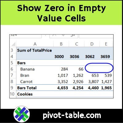
If you build an Excel pivot table, and no data is entered for some items, there will be blank cells in the pivot table values area. See how to change those blanks to zero, or a text string, such as “N/A”
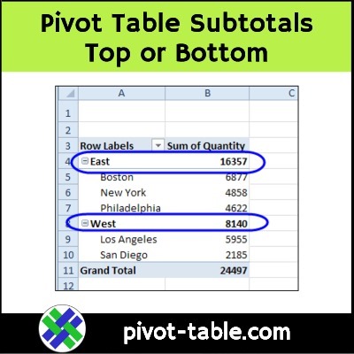
When you create a new pivot table, and add multiple fields to the row or column area, subtotals are automatically created. For Row fields the automatic subtotals usually appear at the top, and you can move them to the bottom, if that’s your preference. There are a few limitations though, which you can see in the video and the written notes below.
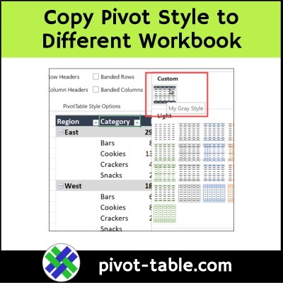
You can create custom PivotTable Styles in an Excel workbook, to fine tune the appearance of your pivot tables. Later, if you want to use those custom styles in a different Excel file, you’ll have to manually copy them, using the steps shown below.
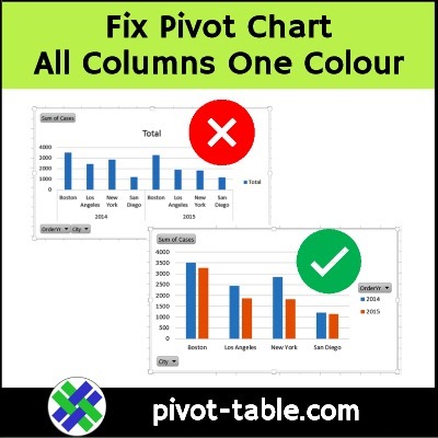
If you make a pivot chart in Excel, you might wonder why all the columns are the same colour. The video below shows a quick fix for that pivot chart problem, and create columns in different colours. Continue reading “Fix Pivot Chart All Columns One Colour”
After you set up a pivot table, you might want to discourage people from filtering the pivot fields, which could hide some of the data. This video shows a couple of ways hide the drop down arrows in the pivot table headings.
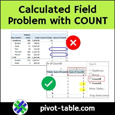
A pivot table calculated field always uses the SUM of other values, even if those values are displayed with another summary function, such as COUNT. That can cause results that look wrong, but the video below shows a workaround to fix the problem.
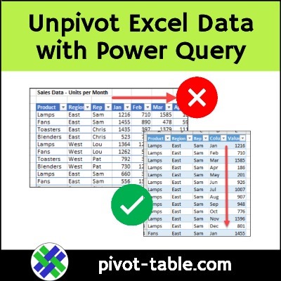
The step-by-step video below shows how to unpivot data in Excel, using Power Query. This creates better source data that you can use to build flexible pivot tables. And this technique doesn’t change your original data!
Pivot tables are a quick way to summarize your data, and they have another advantage too. After you build the pivot table, it’s easy to change the pivot table layout, to get a different type of summary. Watch the two videos below, to see a few examples.
Try Different Pivot Layouts
Pivot tables help you organize and understand your data. They make it easy to summarize tons of information quickly, and you can change the layout to see different types of summaries.
So don’t get stuck in a rut with your Excel pivot tables, by using the same layout, over and over again. Try new things!
After you create a new pivot table, try out different layouts to see which one works best. With just a few clicks, you can tweak the layout of your pivot table to showcase your data in a whole new light.
Tip: Make a copy of the original pivot table worksheet, so you can go back to that version later, if you want to!
To help you get started, here are two videos that show examples of pivot tables in action. Try something different today!
Video: Create Quick Pivot Table and Change Layout
In the video below, you’ll see the steps to create a quick pivot table with Excel’s Recommended Pivot Tables feature.
Then, make simple changes to the layout, to get a different view of your data.
Video Timeline
0:00 Introduction
3:04 Create an Instant Pivot Table
1:26 Pivot Table Field List
2:12 Add and Remove Fields
2:51 Add a Column Field
3:31 Add Another Value Field
4:11 Move the Value Fields
4:55 Reposition the Value Fields
5:15 Change Your Pivot Table
5:30 Get the Sample File
Video: Arrange Multiple Value Fields
If you have 2 or more fields in the Values area of the pivot table, Excel automatically creates a new field in the layout, called “Values”.
Watch this short video, to see how use the Values button, to move the data fields in an Excel pivot table. With these steps, you can change the pivot table layout from vertical to horizontal, or change from horizontal to vertical.
In the screen shot below, the pivot table is in Outline Form layout, and the Value fields have been moved to the Rows area.
Do you love the Excel GetPivotData formula, that appears automatically, when you click on a pivot table value? Or do you want to know how to turn that annoying setting off? In the two videos below, see how to turn GetPivotData off or on, and see an enhanced formula, that pulls data from a specific pivot table in your workbook.
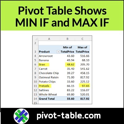
Instead of writing complicated MIN IF or MAX IF formulas in Excel, you can quickly get those numbers in a pivot table. See the easy steps in the video below.