To see the detail behind a number in a pivot table, you can double-click a data cell in the pivot table. This creates a new worksheet, with the related records from the source data. This technique can be helpful when troubleshooting, but you can end up with many extra sheets in your workbook, and you’ll need to delete all the excess sheets.

To avoid all these extra sheets, Héctor Miguel Orozco Díaz has written a macro that applies a filter to your source data, if it is a list in the same workbook as the pivot table.

How The Code Works

The macro applies a filter that is based on the pivot items connected to the cell that you double-clicked. For example, if you double-click the cell circled in screenshot below:

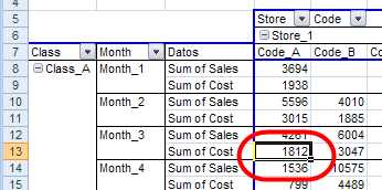
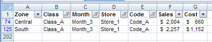
The source data is filtered for Class_A, Month_3, Store_1, Code_A cost, as you can see below.

Download The Sample File

To see Hector’s code and see how it works, you can download the zipped Filter Source Data sample file, or the zipped Filter Source Data sample file - Short with a shorter version of the code.

_________________________