In a pivot table, you can show all the summarized data, or focus on specific details. One way to hide information is with filtering, and that affects the pivot table totals.
Category: Sort and Filter
Block New Pivot Items in Filtered Field
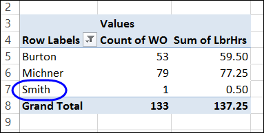
When you click on the arrow in a pivot table heading, you can manually filter the field’s items, by adding and removing check marks from the list of pivot items. That lets you focus the report on specific items, and temporarily ignore the other data.
Change the Report Filter Layout
By default, when you add Report Filters to a pivot table, they are shown in a single vertical list, above the body.

Problems Adding Slicers in Excel 2010
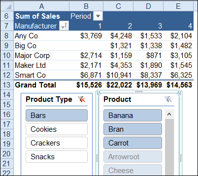
Slicers were introduced in Excel 2010, and they make it easy to filter one or more pivot tables with a single click. In the screen shot below, “Bars” is selected in the product type Slicer. In the Product Slicer, the bars are shown at the top, and the other products are listed below the bars.
Create a Custom List for Pivot Table Sorting
Usually you sort a pivot table’s items alphabetically, or numerically. Here is our current pivot table, with the regions in alphabetical order.

Sometimes you might want another sort order though, such as listing cities or regions in geographical order. In this example, we’d like our company’s regions listed in this order in the pivot table reports – from East to West:
- East
- Central
- West
Creating a Custom List
To show the regions in geographical order, you can create a custom list of regions, in the order in which you want them sorted automatically.
- Click the File tab on the Ribbon, then click Options.
- In the list of categories, click Advanced, and in the General section, click Edit Custom Lists.
- In the Custom Lists dialog box, under Custom Lists, select NEW LIST
- Click in the List Entries section, and type the list of regions, in the order that you want them sorted, pressing the Enter key after each item, to separate the list items
- Click the Add button to add your list to the Custom Lists area
- Click OK twice, to close the dialog boxes.

Sorting with a Custom List
After creating a custom list, the custom sort order isn’t automatically applied to fields that are already in the pivot table layout. You’ll refresh the pivot table to apply the custom list sort order:
- Right-click any cell in the pivot table, and click Refresh.
The regions are then listed in the custom list order.
If the regions don’t automatically change to the custom list order, the field is probably set for Manual Sort. To change the field to Automatic Sort:
- Right-click on one of the region names in the pivot table.
- Click Sort, and then click Sort A to Z

__________________
Hide Drop Down Arrows in Pivot Table Headings
When you add a field to the Row Label or Column Label area of the pivot table, its heading cell shows a drop down arrow. When you click the arrow, you’ll see Sort and Filter options, for the selected field.
In the screen shot below, you can see the sort and filter options for the Product field, and the check boxes for manually filtering the list.

Hide the Arrows
If you want to prevent manual filtering, you can hide the drop down arrows, by using a bit of Excel VBA programming.
The following code will hide the drop down arrow for every field in the first pivot table on the active worksheet.
Sub DisableSelection()
Dim pt As PivotTable
Dim pf As PivotField
Set pt = ActiveSheet.PivotTables(1)
  For Each pf In pt.PivotFields
      pf.EnableItemSelection = False
  Next
End Sub
Sorting and Filtering Still Available
After you hide the arrows, you will still be able to sort the pivot items, by using the commands on the Ribbon.

You’ll also be able to use the Label Filters and Value Filters, if you right-click on an item in the disabled field.

Show the Arrows
After you hide the arrows, you can use similar code to show them again — just change the EnableItemSelection setting to True.
The following code will show the drop down arrow for every field in the first pivot table on the active worksheet.
Sub EnableSelection()
Dim pt As PivotTable
Dim pf As PivotField
Set pt = ActiveSheet.PivotTables(1)
  For Each pf In pt.PivotFields
      pf.EnableItemSelection = True
  Next
End Sub
Video: Apply Multiple Filters to Pivot Field
To see the different types of filters – label, value and manual – please watch this short video tutorial.
Or watch on YouTube: Apply Multiple Filters to Pivot Table Field
________________
Create Worksheet for Each Pivot Item
Last week, Angella emailed me, to ask if there was a way to create a copy of a pivot table, for each item in a report filter.
I suggested that she use a built-in pivot table feature, which is designed to do that – Show Report Filter Pages. The instructions for using this feature are shown below.

However, this built-in feature only copies the pivot table to a new sheet – it doesn’t copy any other content from the original sheet. Angella wanted the pivot table, and she wanted all the other content too.
So, I created a macro that will copy the original sheet, name the copied sheet, and select the pivot item in the copied sheet’s pivot table. You can see the sample code on my Contextures site.
If you just need a copy of the pivot table, you can do the job quickly and easily with the Show Report Filter Pages feature.
Copy Pivot Table with Show Report Filter Pages
To create a quick copy of a pivot table, for each item in a Report Filter field, follow these steps:
- Select a cell in the pivot table (the pivot table must have at lease one Report Filter)
- On the Ribbon, under the PivotTable Tools tab, click the Options tab
- At the left, click Options, then click Show Report Filter Pages
- In the Show Report Filter Pages dialog box, select one of the filters, and click OK
- A new worksheet will be added for each* pivot item, named for the pivot item. (*see exceptions below)
Note: If a sheet with the item’s name already exists, another sheet will be added, with a number added at the end.

Report Filter Page Exceptions
When you run the Show Report Filter Pages command, it might not create a new sheet for each item in the Report Filter. The results will be affected by
- the setting for Select Multiple Items
- which items are currently selected in filter

Select Multiple Items Turned Off
- If (All) is selected, a sheet should be created for each item.
- If a specific item is selected, a sheet will not be created for that item. I guess that Excel assumes that since you already have a pivot table with that item’s data, you don’t need another one.
Select Multiple Items Turned On
- If (All) is selected, a sheet should be created for each item.
- If one item is selected, a sheet will be created for that item only.
- If two or more items are selected (Multiple Items), a sheet will be created for each selected item.
Note: Select Multiple Items is turned off in the pivot table copies, even if it is turned on in the original pivot table.
Use VBA to Copy the Entire Worksheet
If you want to copy all the other content from the original worksheet, along with the pivot table, you can sample code on my Contextures site on my Contextures site. My code adds a “PT_” prefix to the sheets, and deletes any existing “PT_” sheets, if necessary.

___________________
Filter All Pivot Tables for Specific Fields Only
On my Contextures website, there are a few sample files that let you filter one pivot table, and automatically change all the other pivot tables. You can find them on the Sample Files page, in the Pivot Table section.
For example, in the worksheet shown below, if you select Pen Set as the Item in pivot table 1, the same item will be selected in pivot table 2.

This works with Excel VBA Event code, that runs automatically when either pivot table is updated.
Limit the Filter Fields
This code works well, if you want to change all of the fields in all of the workbook’s pivot tables. However, you might have a different worksheet for each Region’s pivot table. If someone changes a Region on one sheet, you don’t want it to automatically change all the other sheets.
In the latest version of the Change Multiple Pivot Tables Automatically workbook, I’ve added a sheet where you can select the specific fields that you want to include. In the screen shot shown below, the Master List pivot table only has Date and Item in its Report Filter area.

Change the Filter
With the revised code, if you filter one of the pivot tables for Region, only that pivot table will be affected, because Region is not in the master list. If you filter for Item or Date, all the pivot tables in the workbook will be updated with the selected item.
In the screen shot below, Region is being changed in the worksheet at the left. The change will not affect the worksheet on the right. However, if the Date is filtered in either pivot table, it will automatically update the other pivot tables in the workbook.

Download the Sample File
To see the code and test the macro, please visit the Excel Sample Files page, and go to the Pivot Tables section. Look for PT0028 – Change Specific Page Fields with Multiple Selection Settings, and download the zipped file.
The file is in Excel 2007/2010 format, and it contains macros. Be sure to enable macros if you want to test the code.
__________________
Create Multiple Copies of Excel Pivot Table
In an Excel pivot table, you can put fields in the Report Filter area, like the City and YrMth fields in the pivot table shown below.

If you need to print a report for a specific city, you can select that city’s name from the drop down list.

Create a Pivot Table for Each City
If you want to print a copy of the pivot table for each city in the drop down list, it might take a while to do the task manually. Instead, you can use a built-in pivot table feature, to automatically create a separate pivot table for each city. Each pivot table will be on its own worksheet, and will have all the formatting that you applied to the original pivot table.
To create a pivot table for each item in a pivot table’s Report Filter:
- In the City filter, select "(All)", or select specific cities from the list. If a city is not selected, a pivot table copy will not be created for it.
- Select a cell in the pivot table, and on the Excel Ribbon, under the PivotTable Tools tab, click
the Options tab. - At the left end of the Ribbon, click the drop down arrow for Options.
- Click Show Report Filter Pages
-

- In the Show Report Filter Pages dialog box, click on City, to select that field.

- Click OK, to create the pivot table pages.
A worksheet is created for each city, with the city’s name on the sheet tab. On each worksheet
is a copy of the original pivot table, with the city’s name selected in the Report Type filter.

Print the City Pivot Tables
After you create the City pivot table pages, you can select all the City worksheets, and print them.
Then, while the City sheets are still selected, delete them, so only the original pivot table is left in the workbook.

More Pivot Table Tips
Please visit the Contextures website for more Excel pivot table tips and tutorials.
________________________
Warning For Excel 2010 Slicers
One of the most useful new tools in Excel 2010 is the Excel Slicer. Add a Slicer to the workbook, and you can filter multiple pivot tables with a single click. Here is a warning for Excel 2010 Slicers though, and if you use the Drill to Details feature