When you create a pivot table, and select a cell in it, a pivot table field list usually appears, at the right side of the Excel window. See how you can adjust that list’s layout, width, and position. Also, see how we moved pivot fields in the olden days – do you remember the PivotTable Wizard?
Here’s a quick trick to add or move Excel pivot table fields, just by typing.
Add or Move Pivot Table Fields
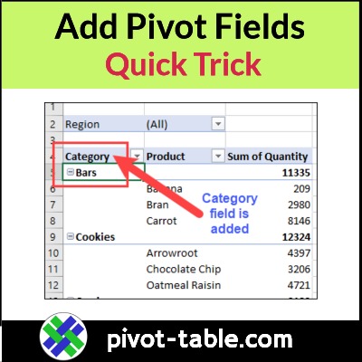
Instead of dragging a pivot field into the layout, you can type its name over an existing pivot field label.
Tip: This is a great shortcut if you like to keep your hands on the keyboard while working in Excel!
Here are the steps to add or move pivot table fields on the worksheet:
First, change the pivot table to Outline layout or Tabular layout. This trick will not work in Compact layout.
Next, click on a cell that contains a pivot field name – a cell where you want a different field to appear
In that cell, type the name of the pivot field that you want to add
Be careful to type the field name correctly
If you make a typo, the field won’t be added
Finally, press Enter, to complete the pivot table layout change
type over pivot field label on worksheet
Pivot Field Added
After you press Enter, the pivot table layout changes.
The field that you typed moves into the active cell.
The existing fields shift down, and the added field takes its new position.
pivot field added to worksheet layout
More Tips for Moving Labels
The first video above shows how to move pivot fields.
You can use a similar trick to move the pivot items in a pivot table.
The short video below shows how to move the Excel pivot items, and you can find written steps on the Move Pivot Table Labels page on my Contextures site.
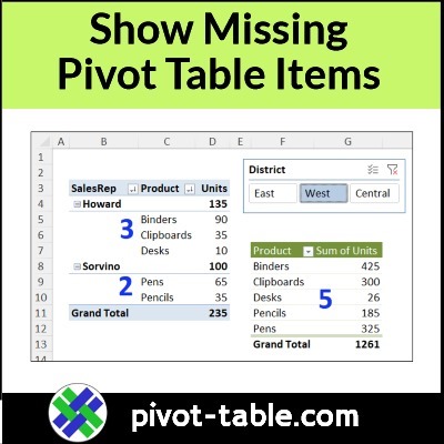
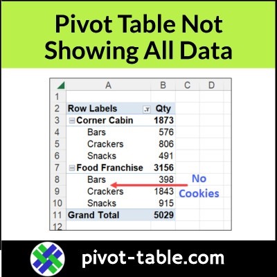
By default, the Pivot Table shows only the items for which there is data. In the example shown in this video, not all colours were sold to each customer. You may wish to see all the items for each customer, even those items with no data.
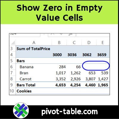
If you build an Excel pivot table, and no data is entered for some items, there will be blank cells in the pivot table values area. See how to change those blanks to zero, or a text string, such as “N/A”
Pivot tables are a quick way to summarize your data, and they have another advantage too. After you build the pivot table, it’s easy to change the pivot table layout, to get a different type of summary. Watch the two videos below, to see a few examples.
Try Different Pivot Layouts
Pivot tables help you organize and understand your data. They make it easy to summarize tons of information quickly, and you can change the layout to see different types of summaries.
So don’t get stuck in a rut with your Excel pivot tables, by using the same layout, over and over again. Try new things!
After you create a new pivot table, try out different layouts to see which one works best. With just a few clicks, you can tweak the layout of your pivot table to showcase your data in a whole new light.
Tip: Make a copy of the original pivot table worksheet, so you can go back to that version later, if you want to!
To help you get started, here are two videos that show examples of pivot tables in action. Try something different today!
Video: Create Quick Pivot Table and Change Layout
In the video below, you’ll see the steps to create a quick pivot table with Excel’s Recommended Pivot Tables feature.
Then, make simple changes to the layout, to get a different view of your data.
Video Timeline
0:00 Introduction
3:04 Create an Instant Pivot Table
1:26 Pivot Table Field List
2:12 Add and Remove Fields
2:51 Add a Column Field
3:31 Add Another Value Field
4:11 Move the Value Fields
4:55 Reposition the Value Fields
5:15 Change Your Pivot Table
5:30 Get the Sample File
Video: Arrange Multiple Value Fields
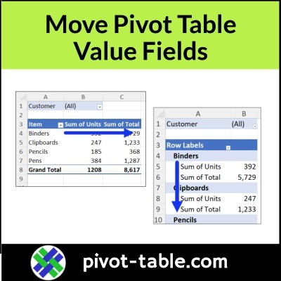
If you have 2 or more fields in the Values area of the pivot table, Excel automatically creates a new field in the layout, called “Values”.
Watch this short video, to see how use the Values button, to move the data fields in an Excel pivot table. With these steps, you can change the pivot table layout from vertical to horizontal, or change from horizontal to vertical.
In the screen shot below, the pivot table is in Outline Form layout, and the Value fields have been moved to the Rows area.
When you create an Excel pivot table, and add values, the value fields are automatically arranged in a horizontal layout, with the headings across the top of the pivot table. To create a narrower, taller pivot table, you can move the Values, so they’re listed vertically. Watch the short video below, to see the steps.
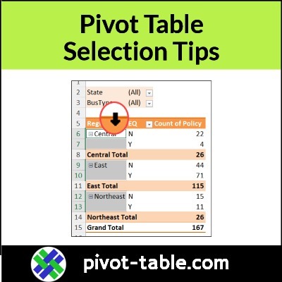
If you’re working with an Excel pivot table, you might want to select a specific section, such as the subtotals, so you can apply formatting. The short video below has a few pivot table selection tips.
Video: Select Specific Parts of Pivot Table
Do you want to select one or two subtotal lines in a pivot table, and change those to a different font or fill colour? Perhaps you want to make one sales region’s totals stand out from the others, in a monthly pivot report.
In this short video, I show how to select specific sections of an Excel Pivot Table, by using the Selection Arrow feature.
And, if the Selection Arrow doesn’t appear on your computer, you’ll see how to turn that feature on, with just a couple of clicks.
Video Timeline
0:00 Introduction
0:15 Pivot Table Selection Arrow
0:47 Select Subtotal Rows
1:06 Select Labels and Values
1:59 Change Enable Selection Setting
More Pivot Table Formatting Tips
Here are a few links to my Contextures site, where you can get more pivot table formatting tips and videos.
Number Formatting: There’s a special way to format numbers in a pivot table, if you want that formatting to stick. If you format pivot table number the same way as normal worksheet cells, the number formatting might disappear, when you refresh the pivot table.
Conditional Formatting: Pivot Table conditional formatting needs an extra step, after you set it up. If you miss that step, new data might not show the conditional formatting!
Pivot Table Styles: An efficient way to format pivot tables is to make changes to the built-in pivot table styles, or create your own custom pivot table styles.
Pivot tables are great for summarizing data, but do you ever notice that there are missing items in a pivot table? For example, you know there are customer records in the source data table, but one customer isn’t showing up in the pivot table. How can you troubleshoot and fix the problem to show all data?
Here’s a quick tip that shows how to remove a pivot table field in Excel. A very short video shows the steps, and there are written steps too, below the video.
Here’s an easy trick to move pivot table fields to a different location in a pivot table, just by typing. See the steps in the short video, and there are written steps below the video, if you prefer those. Continue reading “Easy Trick to Move Pivot Fields”